
Summary
This tutorial describes single site analyses of trial data collected in four different locations. This single site analysis examines the performance of a set of germplasm replicated three times in a balanced incomplete complete block design in each location.
- Introduction
- Select Dataset to Analyze
- Load Data into Breeding View
- Review Results
- Quality Assurance
- Report
- Heritability Table
- Combined File of Predicted Means
- Individual Environment Reports
- Environment Report Summary
- Genotypes by Environment Sorted by BLUPs
- Summary of Traits by BLUP
- Genetic Correlations Between Traits
- Summary Statistics for Individual Trait Raw Data
- Estimated Heritability of Individual Trait
- Genotypes by Trait Sorted by BLUEs
- Standard Errors of Difference
- Wald/F Test
- Diagnostic Residual Plots of Individual Traits
- Upload BLUEs & Summary Stats to BMS
- References
- Related Materials
Introduction
Breeding View’s single site analysis produces adjusted means, best linear unbiased estimators and best linear unbiased predictors (BLUEs and BLUPs) per genotype, as well as summary statistics to describe the data. The next tutorial, Multi-Site (GxE) Analysis, uses the summary statistics and adjusted means (BLUEs) to perform a genotype by environment (GxE) analysis. Adjusted means can also be used in a QTL (quantitative trait loci) analysis pipeline.
Select Dataset to Analyze
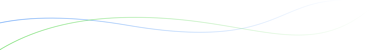
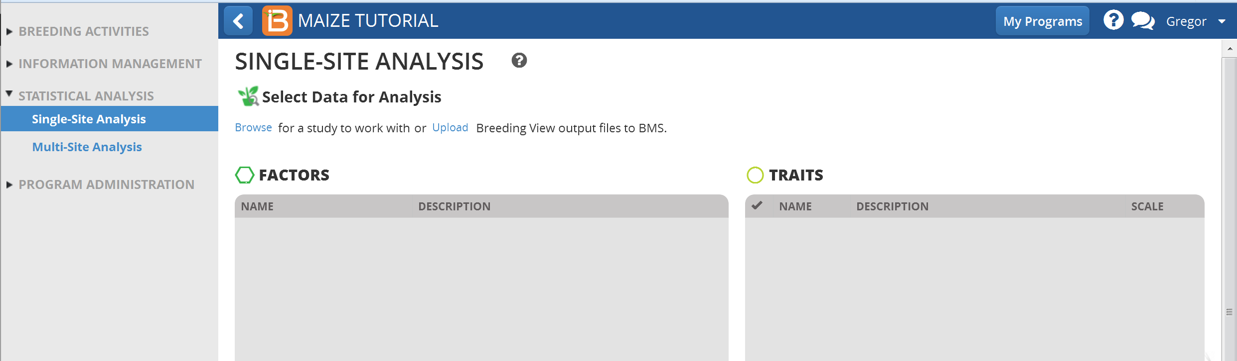
- Open Single Site Analysis from the Statistical Analysis menu of the Workbench. Select Browse to find the 4 Location Trial dataset.
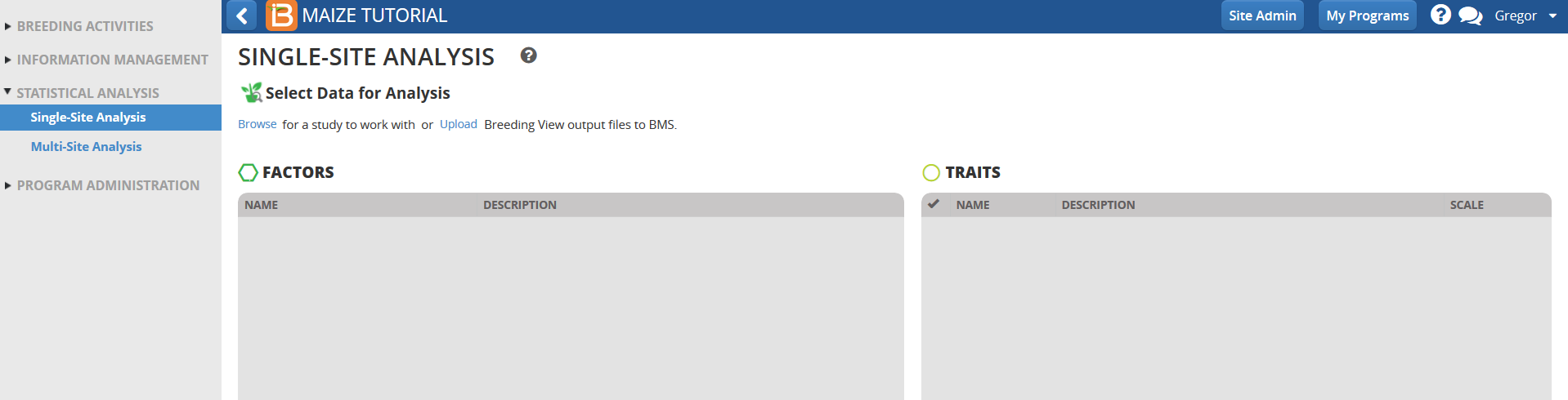
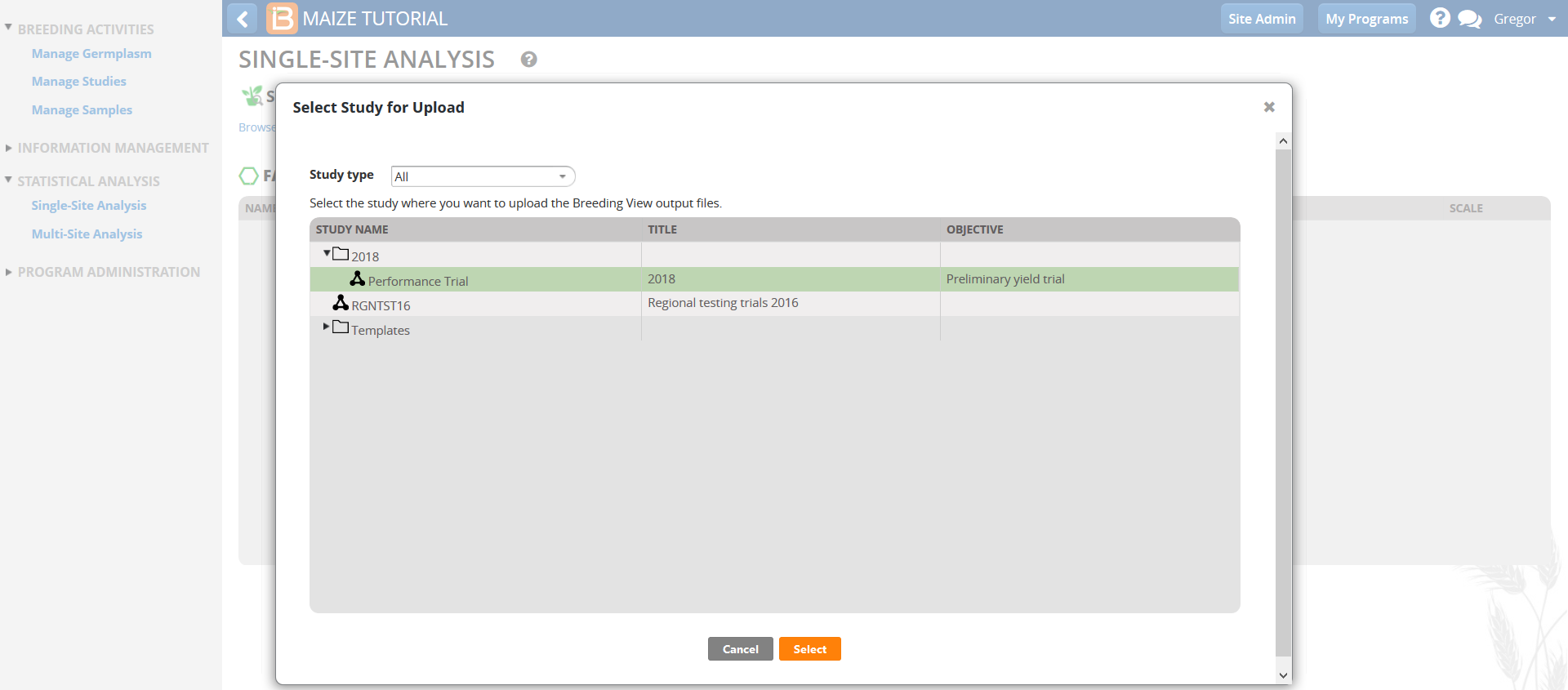
- Select 2018 Performance Trial.
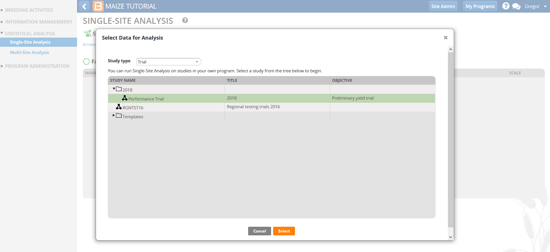
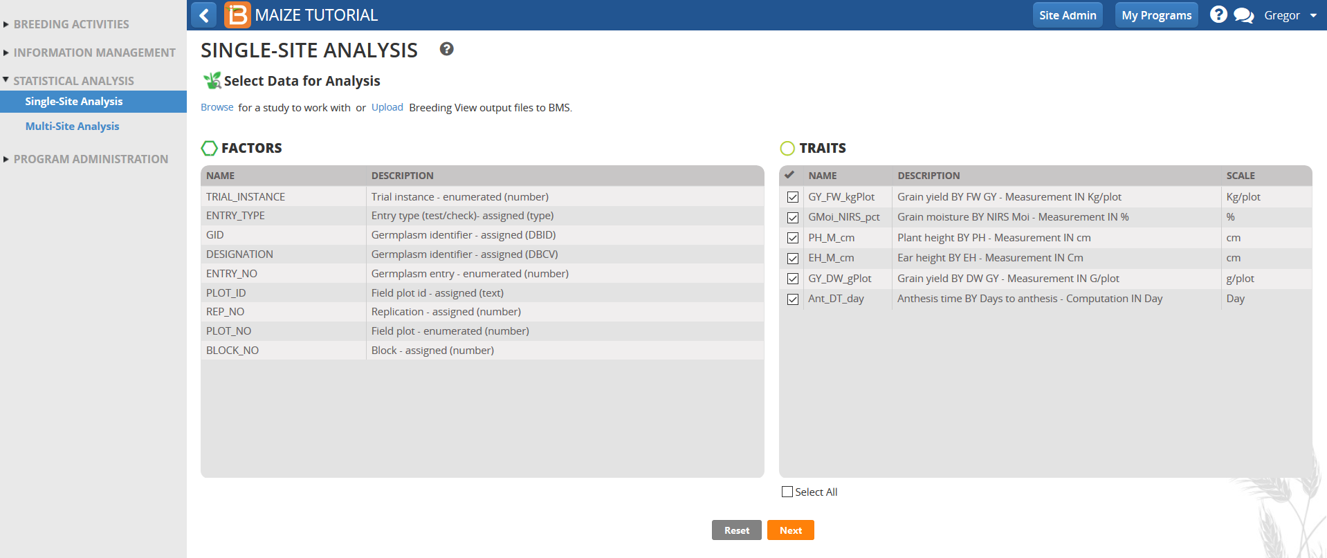
- Review the factors and make sure the six phenotypic traits measured in this trial dataset are selected, and click Next.
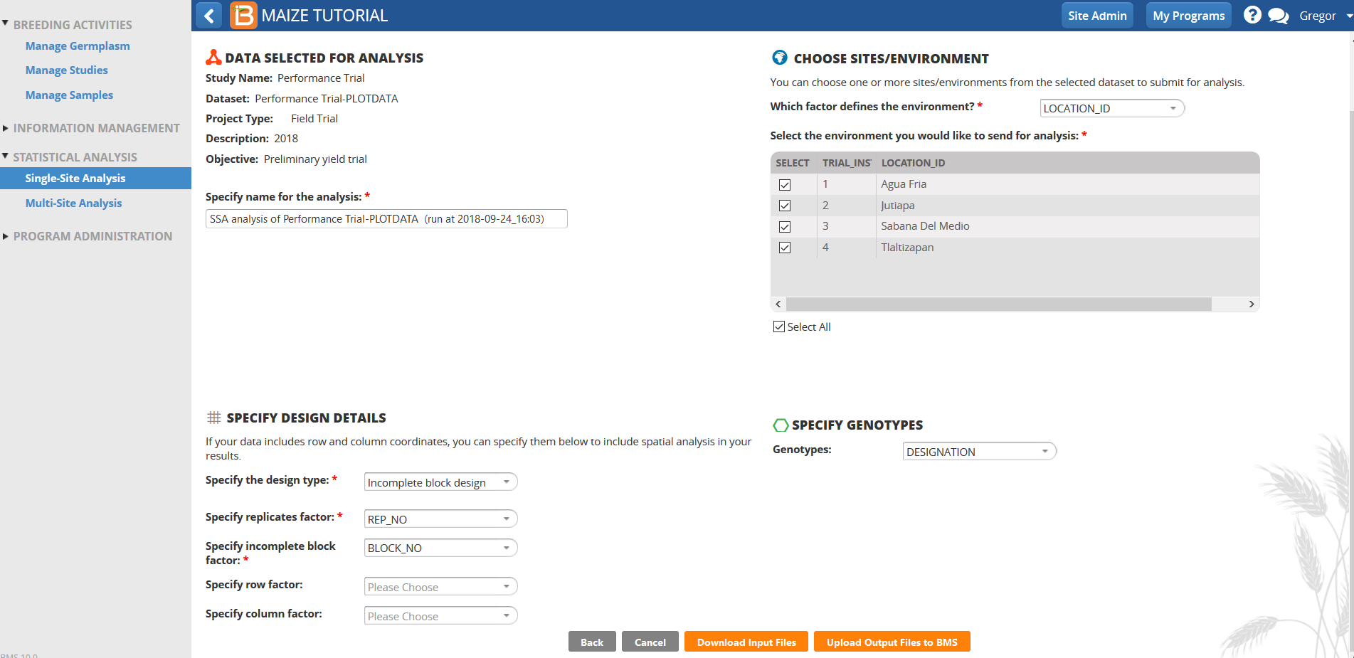
- Specify Analysis Conditions
- Use the default analysis name.
- In the Specify Design Details window, Select Incomplete Block Design for the design type.
- REP_NO is the factor in this dataset that defines replications.
- BLOCK_NO is the factor that specifies the Incomplete Block factor
- In the Specify Genotypes window, select DESIGNATION as the factor that defines the Germplasm to be used in the analysis.
- In the Choose Sites/Environment window, select LOCATION_ID as the factor that defines environments.
- Select the 4 locations to perform 4 individual single site analyses.
- Specify row factor and Specify column factor windows should be left blank for this trial.
- Select Download Input Files.
Load Data into Breeding View
BMS Version 10.0 is a server application. Breeding View (BV) is a Windows compatible desktop application (see Install Breeding View). Trial data exported from the BMS are perfectly formatted for analysis by the BV application.
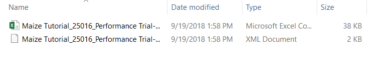
- Decompress, or unzip, the input folder to reveal the two files for input into the Breeding View application.
- Launch the Breeding View application on your local computer and select Open Project.
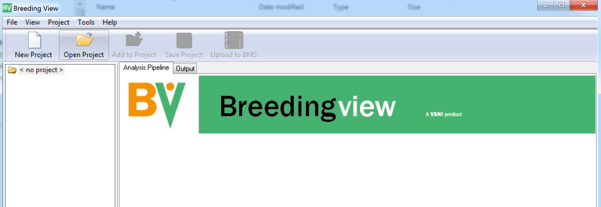
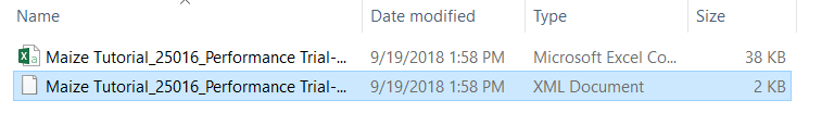
- Load trial details into the Breeding View application. Browse to the .xml file and open.
Run Analysis
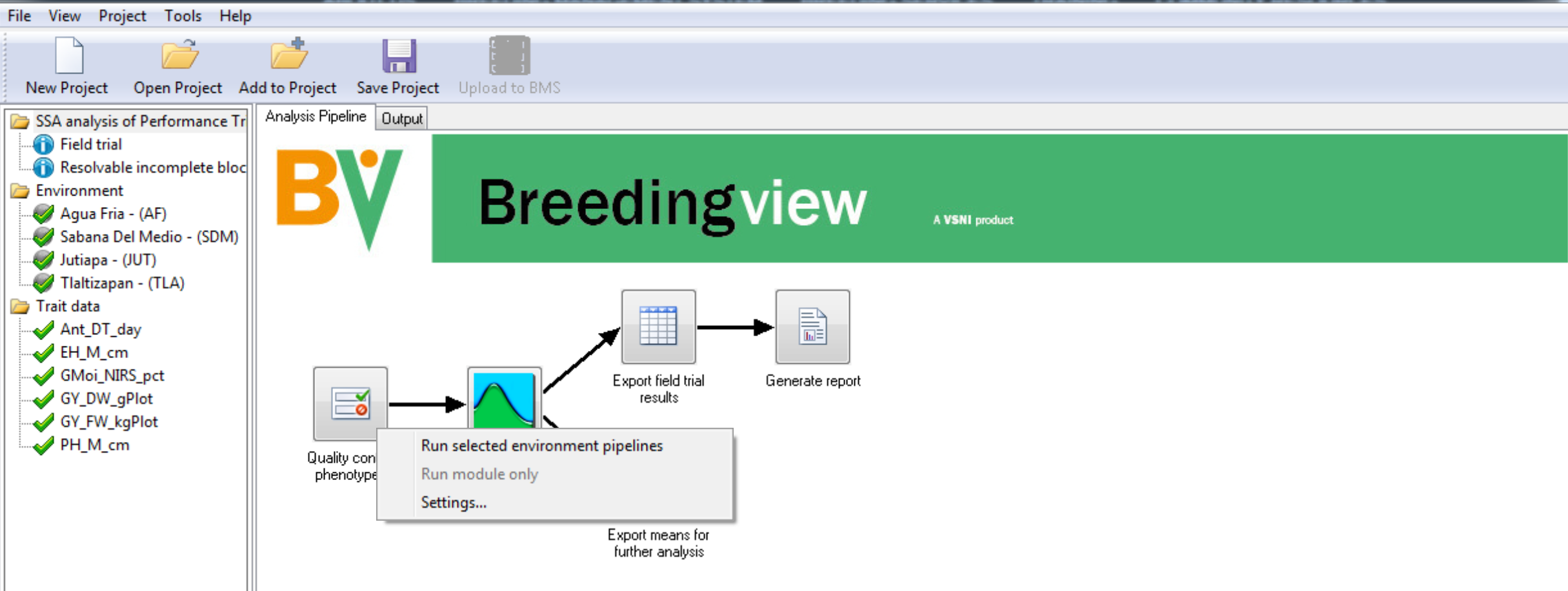
The analysis pipeline includes a set of connected nodes, which can be used to run and configure pipelines.
- Right click on the Quality Control Phenotypes. Run the analysis pipelines for the selected 4 environments.
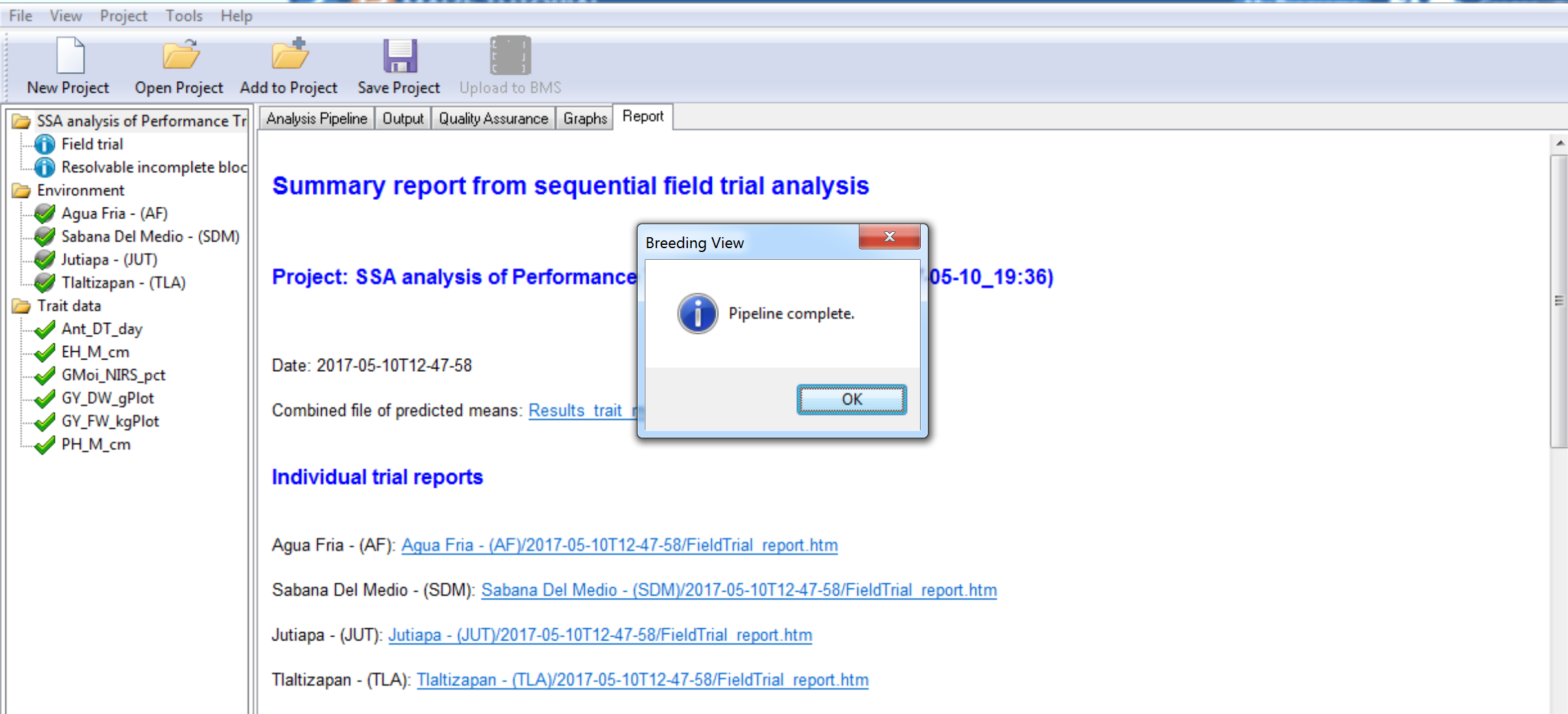
When the analysis is complete a popup notifies the user.
- Select OK to view the analysis results.
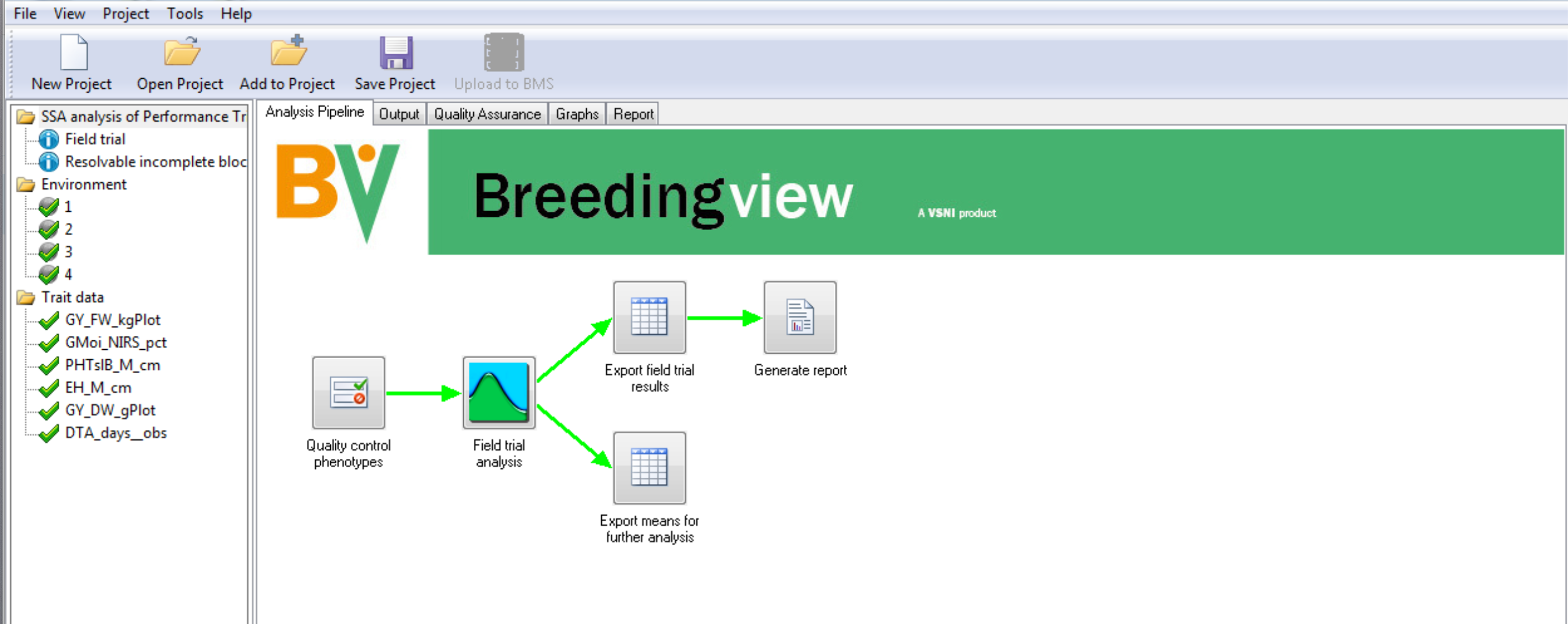
All of the nodes in the analysis pipeline are green when the analysis are complete.
- Select the Quality Assurance tab.
Review Results
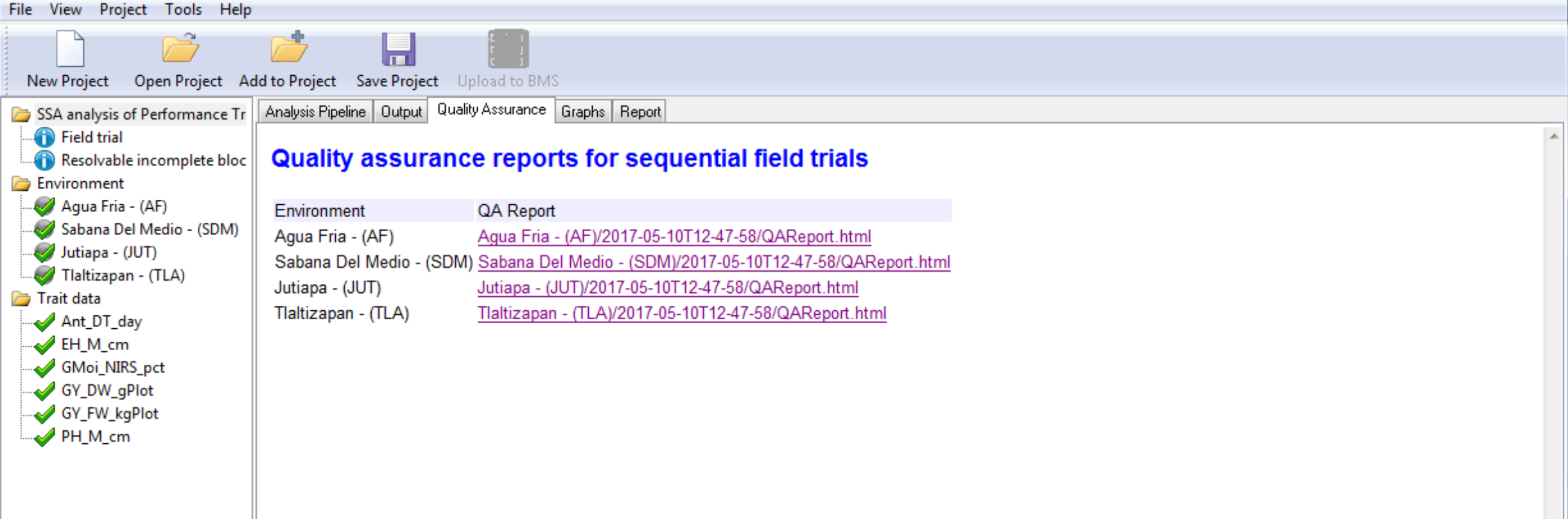
Quality Assurance
Breeding View provides an overview of potentially influential measurements to help users identify and possibly exclude observations. Influential observations may reflect true genotypic variation and care should be taken not to exclude these data from the trial. Observations that deserve exclusion are obvious errors or measurements influenced by heterogeneous environmental variation within a block, like damage to a single plot.
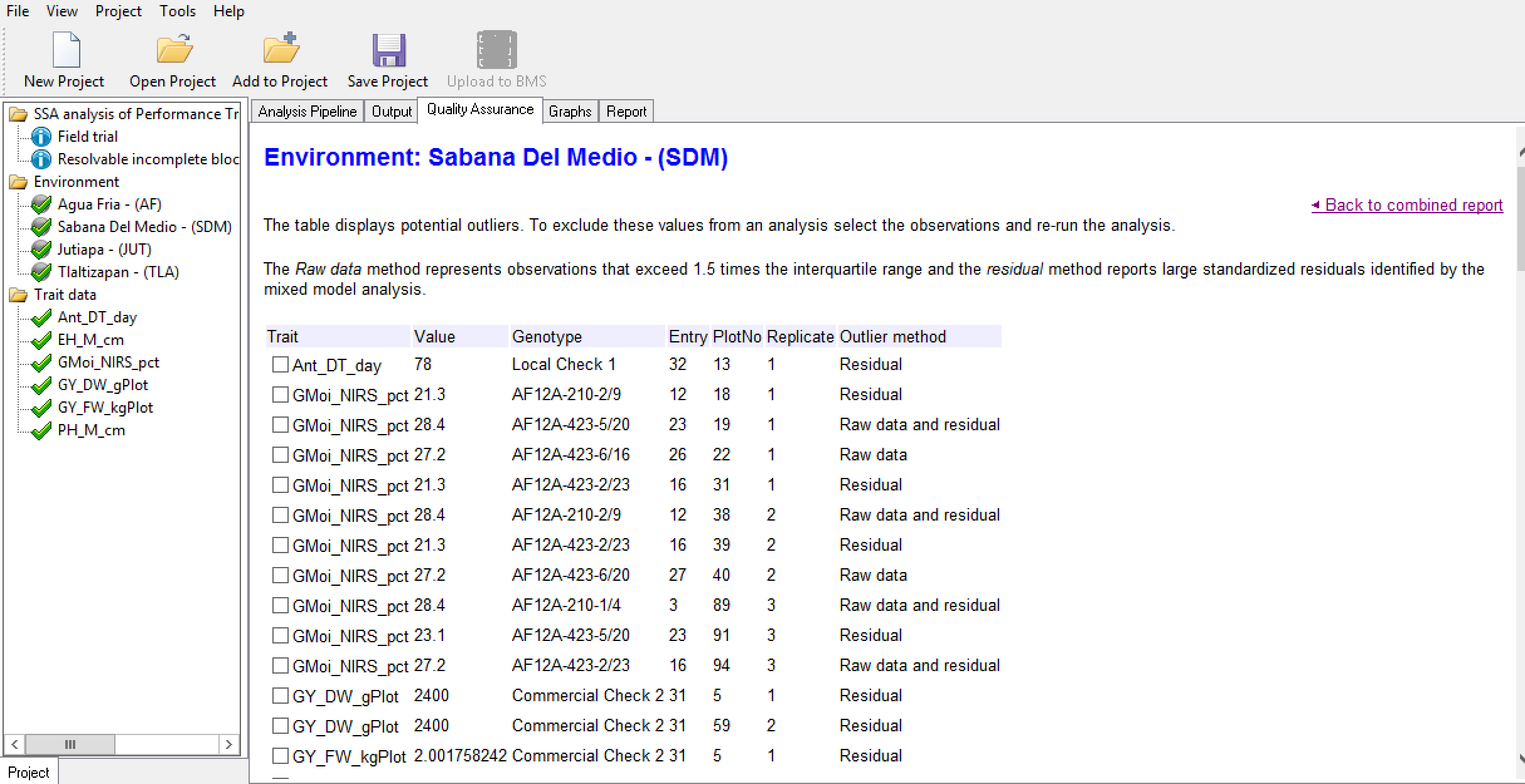
- Select and open the report of the trial conducted at Sabana Del Medio.
The table displays potential influential observations identified by the raw data method, which identifies observations exceeding 1.5 times the interquartile range, and the residual method, which identified standardized residuals by mixed model analysis. Checking the box by entry allows you to exclude that value from the analysis.
Box plots are provided to graphically illustrate influential measurements.
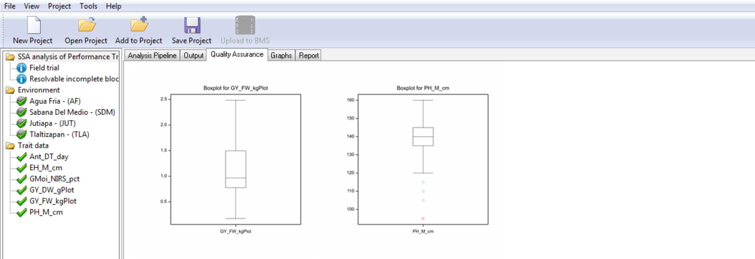
Notice that plant height (PH_M_cm) has a potential outlier measurement highlighted in red.
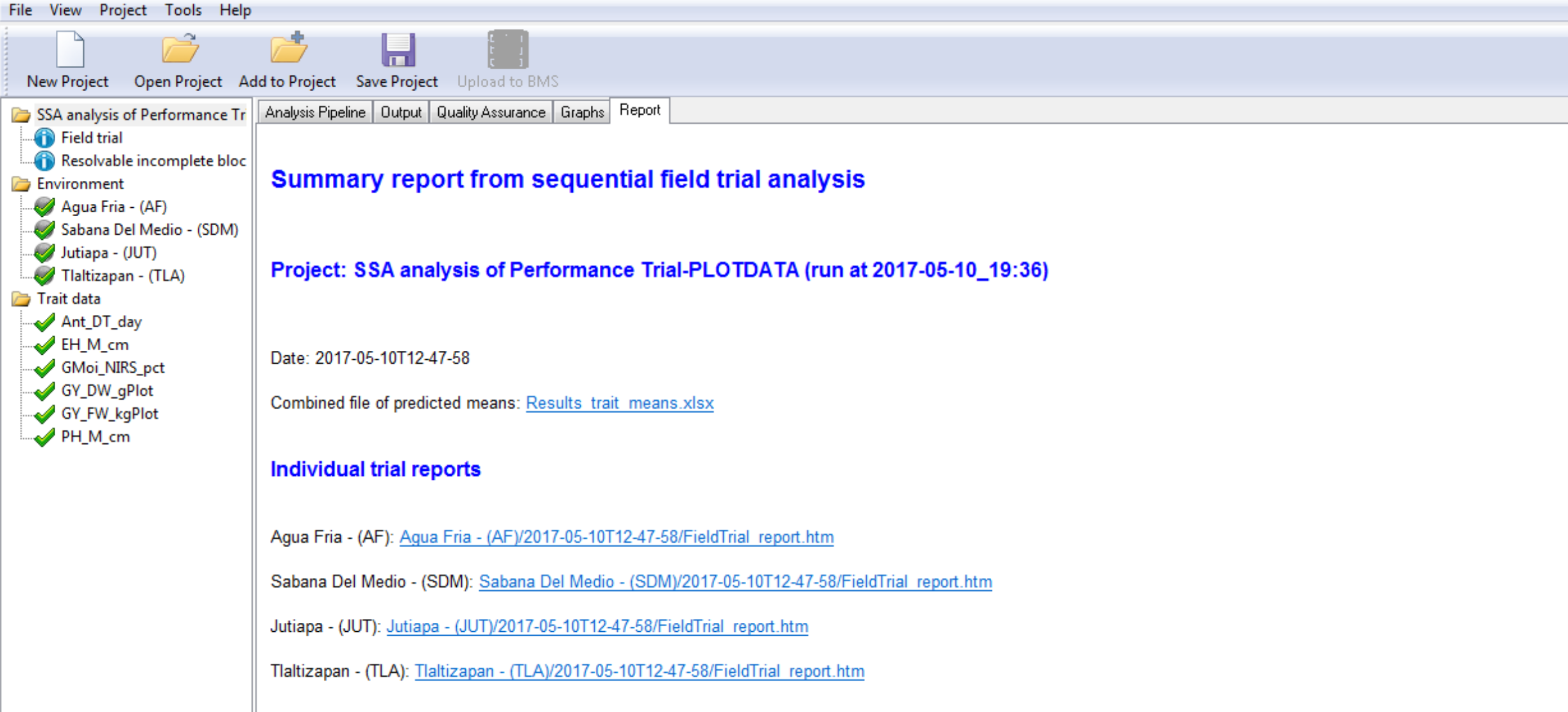
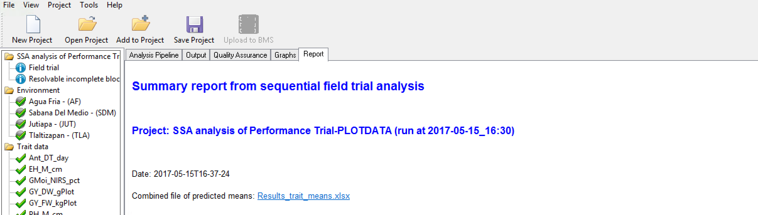
Report
This section of the tutorial provides a brief guide to interpretation of the results, including graphs, included under the Report tab.
Report Tab Contents
- Heritability Table
- Combined File of Predicted Means: Excel file of BLUEs and BLUPs
- Links to Individual Environment Reports
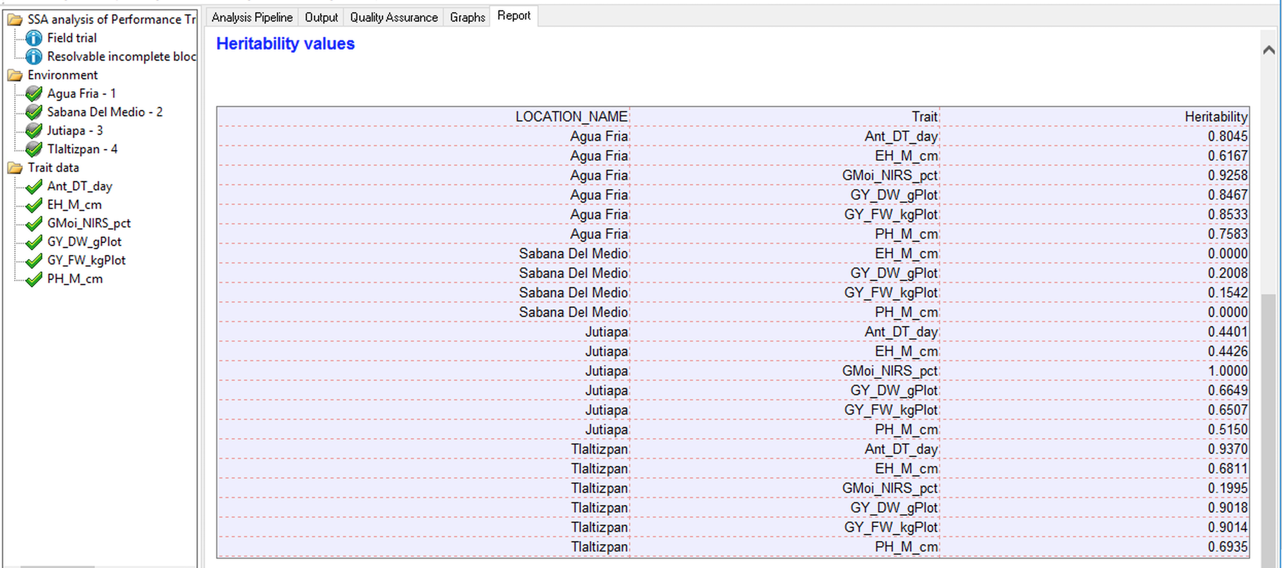
Heritability Table
The heritability table summarizes the generalized heritabilities calculated for each trait by location as described by Oakey et al. 2006. The method uses the average pairwise prediction error variance to obtain genetic and error covariance matrices and allows for the estimation of heritability in unbalanced data with complex error and genetic structures. If a model cannot be fitted to the trait data, such as when there is no variability in the trait measurement, that trait will not be included in the heritability table.
Combined File of Predicted Means
- Select the link to the combined file of predicted means.
- Open in Excel. Non-informative traits that could not be fitted with a model will appear as missing data.
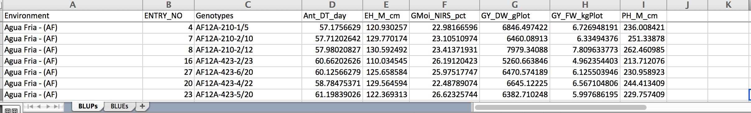
BLUPs across all locations
Breeding View reports BLUPS and BLUES for each entry in each location. BLUES (Best Linear Unbiased Estimates) are the classical least squares means from the fixed effect model, and BLUPS are the Best Linear Unbiased Predictors from a mixed model in which the entries are modeled as a random effect. BLUES suffer a disadvantage in predicting future performance of an entry because extreme values can result from a good genotype or a lucky environment (eg extra fertile plot). Mixed models estimate the variability of these two components - genotypes and environment, and adjust the means towards the grand mean by an amount which depends on the ratio of genetic to total phenotypic variance (the heritability). If this ratio is large, near 1, the adjustment is very small and BLUES and BLUPS will be almost the same, but if this ratio is small, near 0, the adjustment will be large and BLUPS for all entries will be about the value of the grand mean. BLUPS have been empirically shown to be much better predictors of future performance than BLUES, and the heritability (more accurately described as the repeatability) measure presented is a very good guide to the value of the results of each location in terms of distinguishing between the genetic merit of the entries. If heritability is moderate to low users should be guided in their selections by the BLUPS, in cases of high heritability there is little difference.
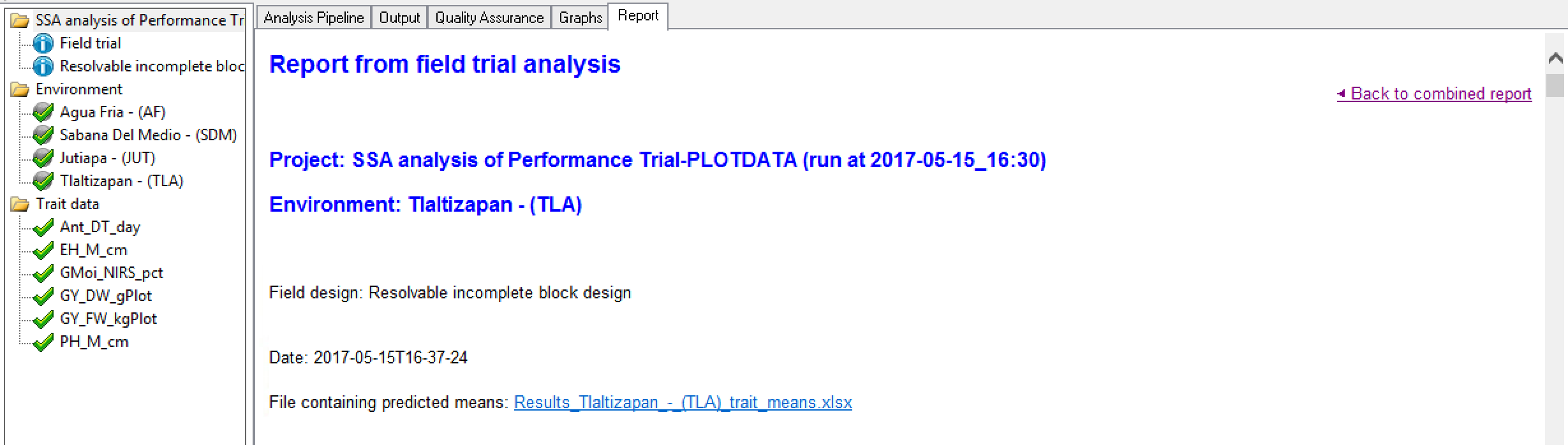
Individual Environment Reports
Although the four locations are summarized together in the table, each location is represented by an individual analysis. Select the link to the Environment 4 individual trial report to review the analysis performed at this location.
Individual Environment Reports Include:
- File of predicted means: Link to Excel (.xls) file containing an environment-specific subset of BLUEs and BLUPs
- Best Genotypes Table: Best genotypes as defined by BLUPs sorted by factors defined in the report options
- Summary of Traits: A table presenting the minimum, mean, maximum, and heritability for each trait within this location based on BLUPs
- Estimated Genetic Correlations Between Traits
- Principle Components Biplot
- Individual Trait Analysis: Summary statistics of raw data, heritability, sorted genotype table (BLUEs), standard errors of differences, and residual diagnostic plots.?
Environment Report Summary
The environment report provides the project name, the environment name, the field design, along with a date the stamp for the analysis. Users are presented a link to the adjusted means data for this environment, which is a subset of the data presented in the combined mean file reporting all locations. The file reports the BLUPS and BLUES for each entry on separate sheets (see details above). Users are also notified about analysis failures.
This file also contains summary statistics which are sometimes a little different from those computed from older statistical packages. This is because they are computed from results of different models - mixed models, which are more suited to representing field trial data and are now available to us with the new computing algorithms available in Genstat and Breeding View. For example, for the CV Breeding View uses 100 x sqrt (estimated residual m.s.) / (estimated grand mean), where the residual sum of squares is estimated from fitting the FIXED model by GLS with a covariance matrix derived from the estimated variance components. The estimate grand mean is calculated by taking the mean of the fitted values and the heritability is the generalised heritability which is different to the simple heritability calculation of Var(G)/Var(P) which is adequate for simple models, but not for more complex ones such as spatial models. Generalized heritability is described in Oakey et al. 2006 and Cullis et al. 2006.
Genotypes by Environment Sorted by BLUPs
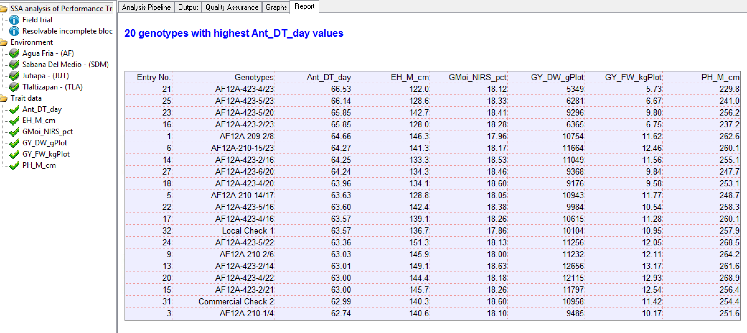
20 Best Genotypes at Tlaltizapan Sorted by Days to Anthesis: This table is the 20 best genotypes sorted by BLUPs for days to anthesis in descending order, as defined by the settings under the Generate Report node. Note that while breeders generally select for high phenotypic values, days to anthesis is an exception - delayed maturity is generally selected against.
Summary of Traits by BLUP
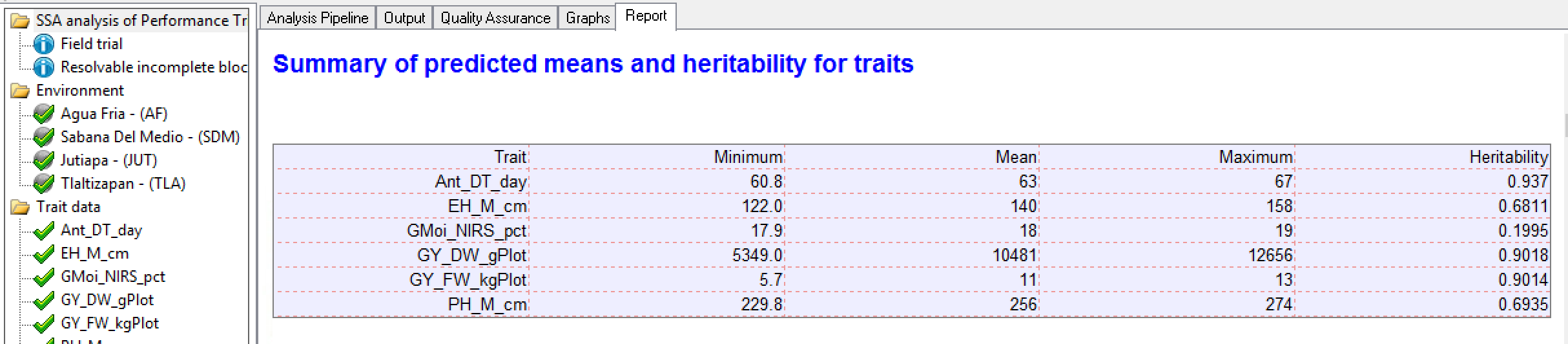
Tlaltizapan Summary of Traits: The minimum, mean, maximum, and heritability for each trait based on BLUPs
Genetic Correlations Between Traits
BLUPs Principle Components Biplot
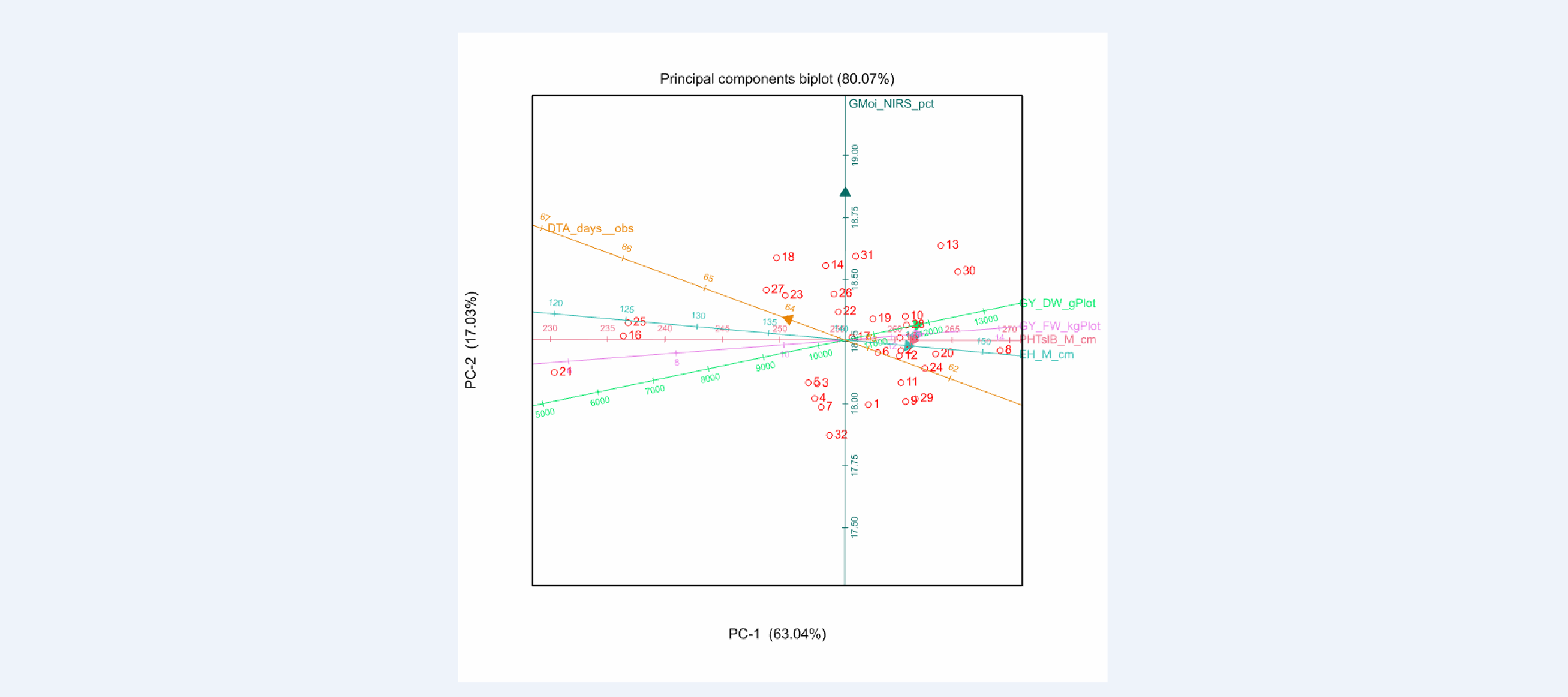
Tlaltizapan Principle Components Biplot of BLUPs:The biplot shows that field weight, grain yield dry & fresh weight (GY_DW_gPlot & GY_FW_kgPlot), plant height (PHTsIB_M_cm) , and ear height (EH_M_cm) are all positively correlated among each other (acute angle of vectors), and negatively correlated with anthesis date (DTA_days_obs) (obtuse angle). In addition, all traits are weakly correlated with grain moisture (GMoi_NIRS_pct) (right angle). These relationships can also be seen in the genetic correlation matrix below.
Genetic Correlation Matrix
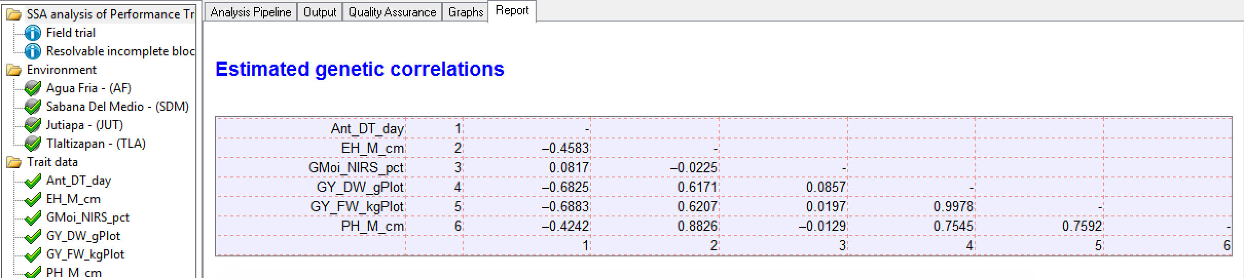
Tlaltizapan Estimated Genetic Correlations: Pairwise correlation (r) of phenotypic traits. There is a strong positive correlation (0.9978) between the related yield measures, grain yield and field weight (GY_DW_gPlot & GY_FW_kgPlot). These two yield traits are moderately negatively correlated (-0.6890 & -0.6830 respectively) to anthesis date (Ant_DT_days). In other words, late anthesis is correlated to low yield.
Summary Statistics for Individual Trait Raw Data
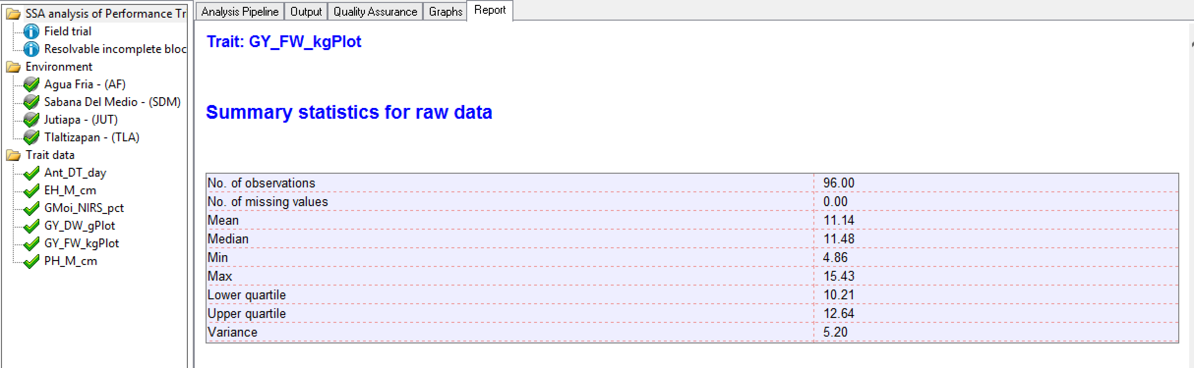 Tlaltizapan Summary Statistics for Grain Yield (GY_FW_kgPlot) based on raw data
Estimated Heritability of Individual Trait
BV reports the generalised heritability. This is different to the simple heritability calculation of Var(G)/Var(P) which is adequate for simple models, but not for more complex ones such as spatial models. Generalized heritability is described in Oakey et al. 2006 and Cullis, Smith and Coombes, 2006.
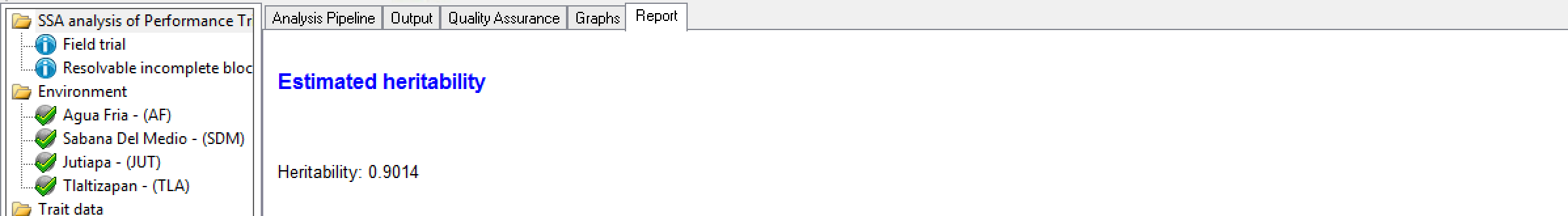 Estimated Heritability of Grain Yield (GY_FW_kgPlot) calculated at Tlaltizapan
 Genotypes by Trait Sorted by BLUEs
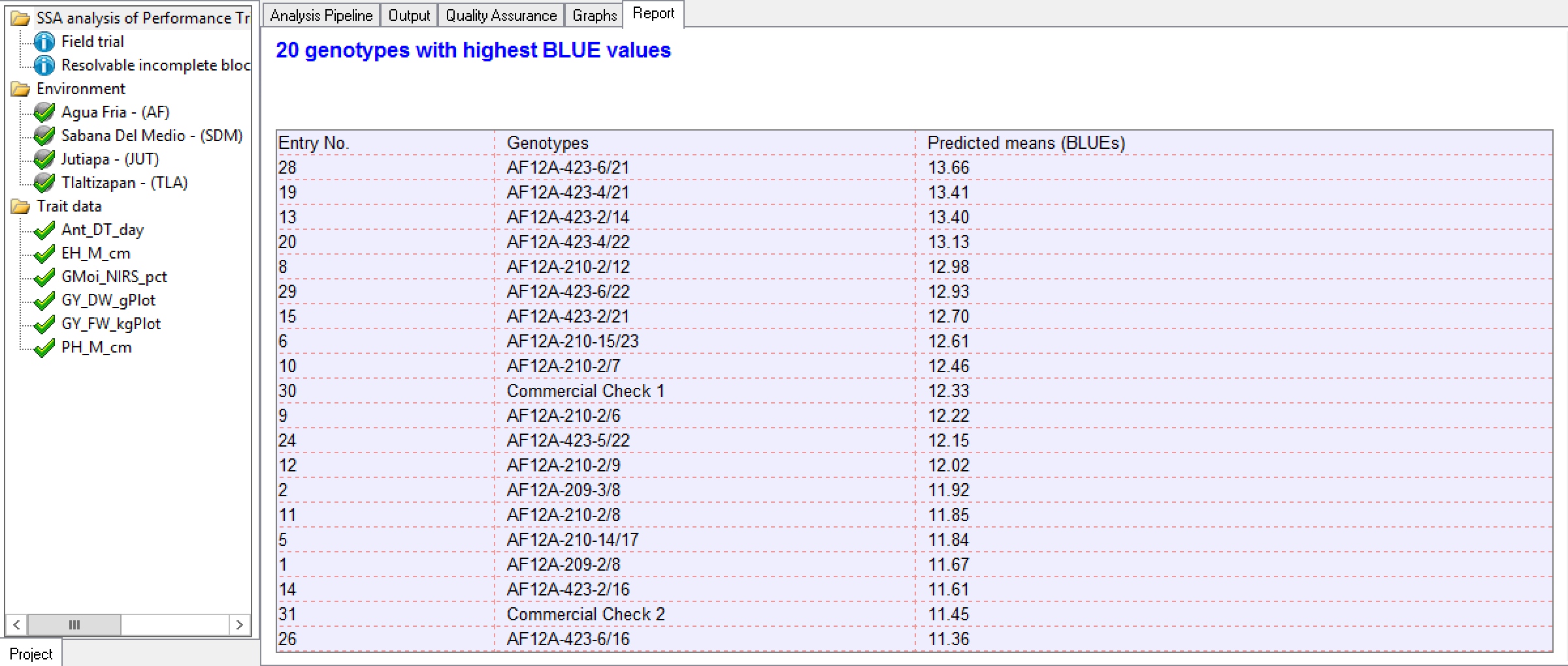 20 Best Grain Yield (GY_FW_kgPlot) Genotypes Calculated at Tlaltizapan: Genotypes are sorted by BLUEs in descending order by value as specified in the Report Options.
Standard Errors of Difference
Two genotypes are considered different when their means are 2 times the standard error of the difference (SED), equivalent to LSD (Least Squared Difference). In general a breeder would use the average, and consider the minimum and maximum to have some sense of the differences in precision of comparisons among means.
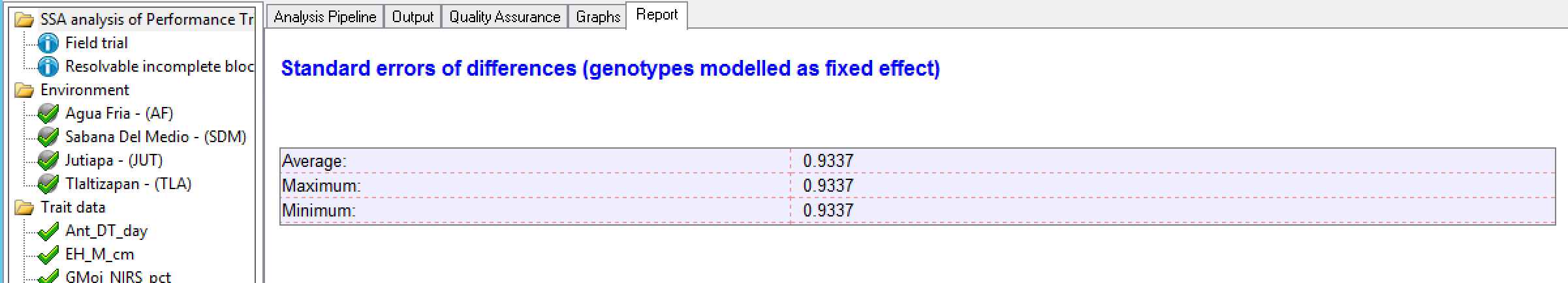
Standard Errors of Difference for Grain Yield (GY_FW_kgPlot): In a balanced design without missing data, like in this example the average, maximum, and minimum SED are equivalent.
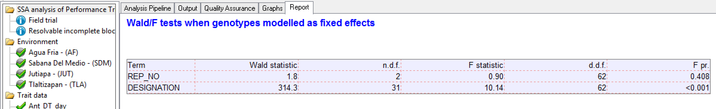
Wald/F Test
Diagnostic Residual Plots of Individual Traits
Diagnostic residual plots are used to check the model assumptions. Residuals are defined as the difference between the observed and fitted values. A good model “fit” for adjusted means will have residuals that should be independent and follow a normal distribution with a mean of zero and a constant variance. All but the independence assumption can be checked with the residual plots - independence follows from the randomization of the experimental design.
Utility of Each Diagnostic Plot
- Histogram of Residuals: Check for a normal, or Gaussian distribution, as well as centering on a mean of zero.
- Fitted-Value Plot: Check for constant variance as well as centering on zero. A random distribution, or “shot-gun pattern”, reflects constant variance. Positive or negative correlations between residuals and fitted values, or ‘loud-speaker-shaped’ distributions, point to violation of the constant variance assumption
- Normal Plot: Check normality. Distribution in a straight line across the diagonal reflects a normal distribution. The Normal Plot has the same use as the Histogram of Residuals, but is generally a better visualization.
- Half-Normal Plot: Check normality. Distribution in a straight line across the diagonal reflects a normal distribution. The Half-Normal plot is the same as the normal plot, but considers the absolute value of residuals. This plot is useful with small data sets.
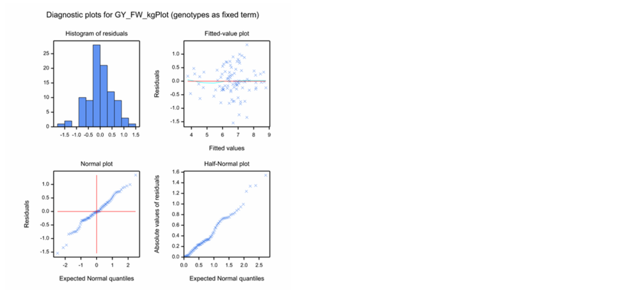
Diagnostic plots for Grain Yield (GY_FW_kgPlot) in Tlaltizapan: Example of a continuous variable exhibiting a good model fit
Upload BLUEs & Summary Stats to BMS
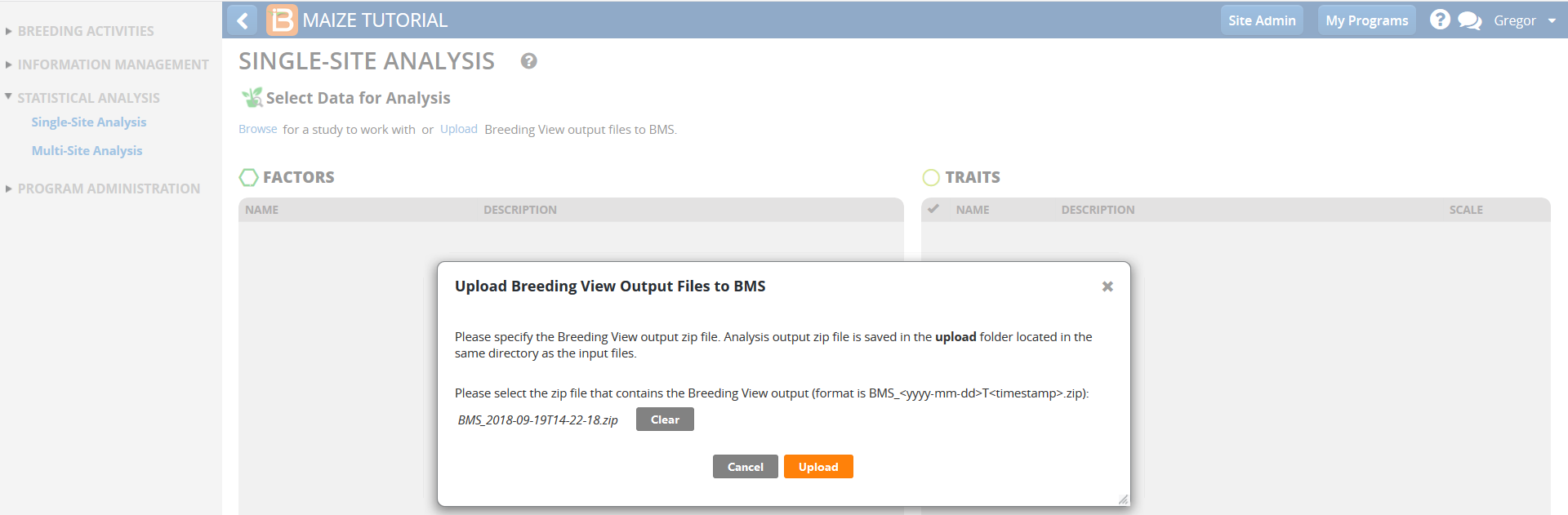
- Return to the Breeding Management System Single-Site Analysis. Select Upload Breeding View Output Files to BMS to save the adjusted means and summary statistics to the BMS database for use in the subsequent Multi-Site (genotype by environment) analysis.
- Highlight the Performance Trial 2018 and Select.
- Select Browse.
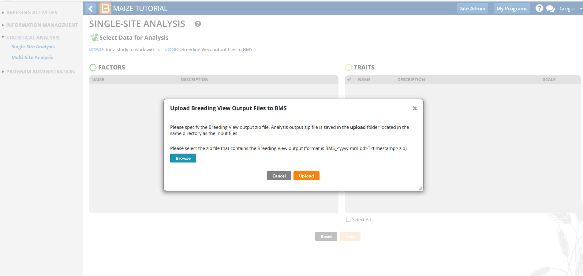
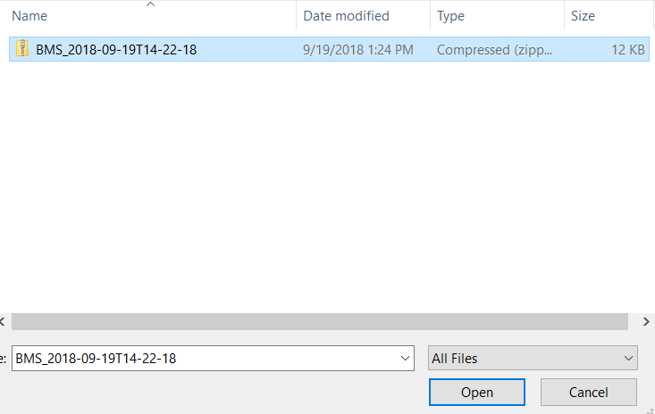
- Browse to the zipped Breeding View Upload file in your computer. The zip file is date and time stamped, and can be found within the upload folder. Select the zip file and upload.
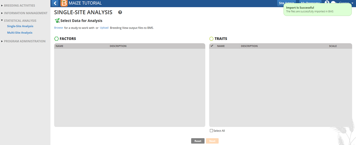
Once the import is successful, the means and summary statistics from the single site analysis are available to perform a Multi-Site (genotype by environment) analysis.
- Confirm the uploaded SSA analysis data by selecting the Performance Trial from the Browse Studies menu option in the INFORMATION MANAGEMENT Tool.
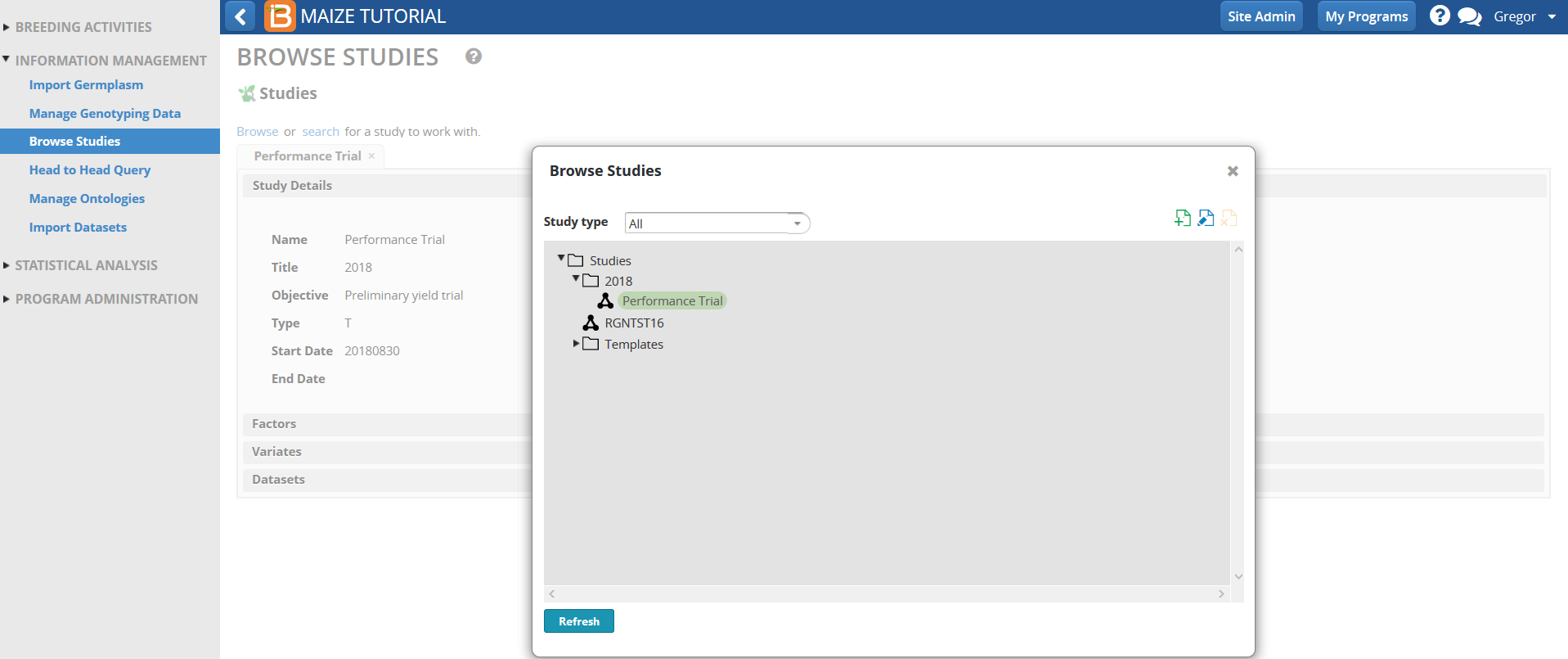
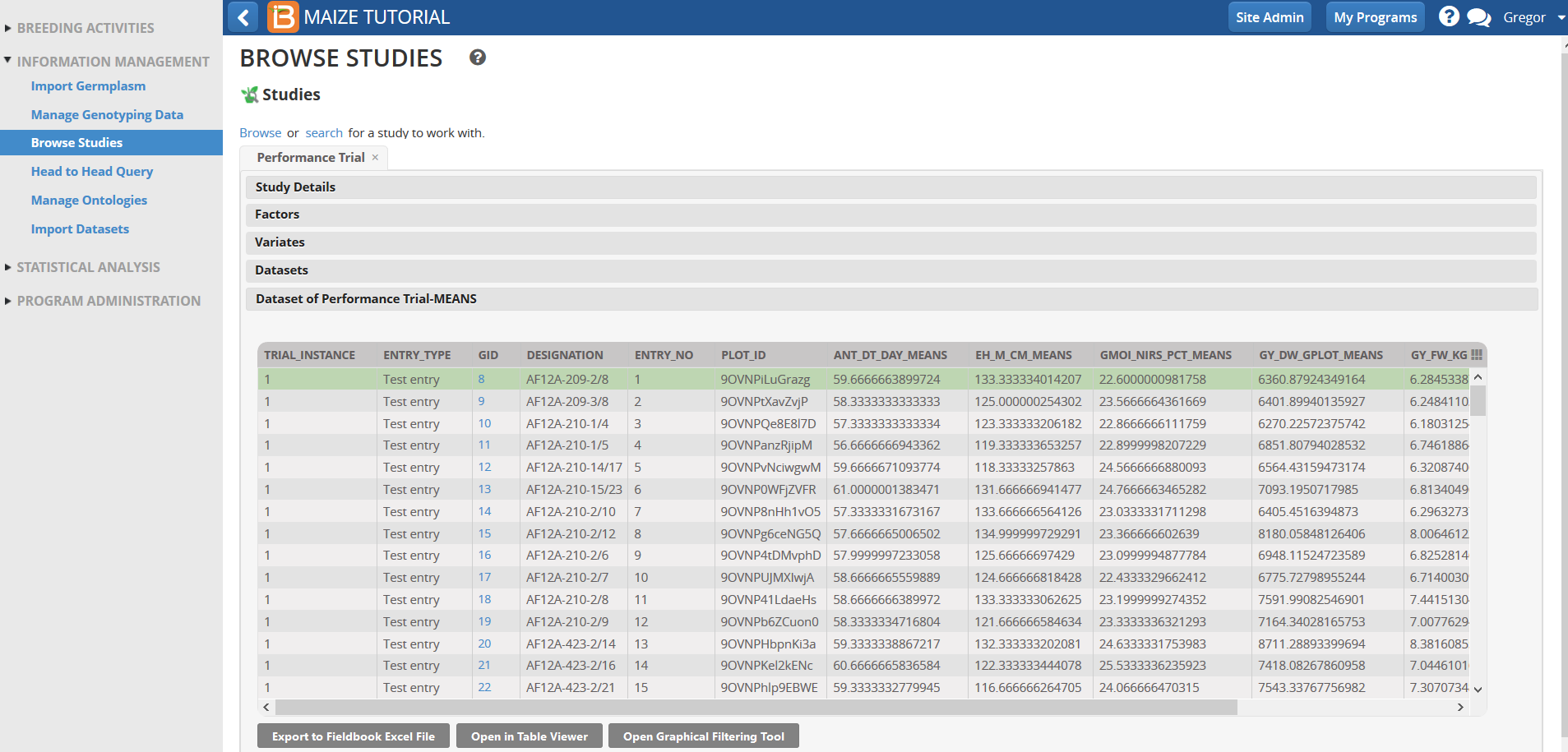
- Select Datasets and highlight Performance Trial MEANS dataset.
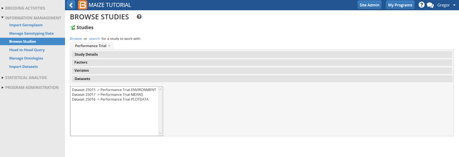
Scroll down and review the Means data for different traits for the four environments (Trial instances).
References
Cullis, Smith and Coombes, 2006. On the Design of Early Generation Variety Trials With Correlated Data. American Statistical Association and the International Biometric Society Journal of Agricultural, Biological, and Environmental Statistics, Volume 11, Number 4, Pages 381–393. DOI: 10.1198/108571106X
Oakey, H., Verbyla, A. P., Pitchford, W., Cullis, B., & Kuchel, H. (2006). Joint modeling of additive and non-additive genetic line effects in single field trials. Theoretical and Applied Genetics, 113, 809–819.
Murray, D. Payne, R, & Zhang, Z. (2014) Breeding View, a Visual Tool for Running Analytical Pipelines: User Guide. VSN International Ltd. (.pdf) (Sample data .zip)
Related Materials
BMS Manual
Manage Trials
Install Breeding View
Maize Tutorials
Trial Design & Planting
Trial Data Collection
Single Site Analysis
Multi-Site Analysis
Funding & Acknowledgements
The Integrated Breeding Platform (IBP) is jointly funded by: the Bill and Melinda Gates Foundation, the European Commission, United Kingdom's Department for International Development, CGIAR, the Swiss Agency for Development and Cooperation, and the CGIAR Fund Council. Coordinated by the Generation Challenge Program the Integrated Breeding Platform represents a diverse group of partners; including CGIAR Centers, national agricultural research institutes, and universities.
The statistical algorithms in the Breeding View were developed by VSN International Ltd in collaboration with the Biometris group at University of Wageningen. Maize demonstration data was provided by Mike Olsen from the CIMMYT, the International Center for Maize and Wheat Improvement, breeding program. These data have been adapted for training purposes. Any misrepresentation of the raw breeding data is the solely the responsibility of the IBP.

This work is licensed under a Creative Commons Attribution-ShareAlike 4.0 International License
