
 ?
?
Image Credit: http://phymap.ucdavis.edu/cowpea/
Contributors
Shawn Yarnes a, Darren Murray b, Roger Payne b & Zhengzheng Zhang b
?a The Integrated Breeding Platform, b VSN International Ltd
Summary
This tutorial provides instruction on the analysis of genotype by environment (GxE) interactions within a three-location cowpea field trial. This tutorial builds upon the adjusted means calculated for the individual locations in the previous tutorial, Single Site Analysis: 3 Location Batch.
- Restore from Previous Tutorial
- Introduction
- Select Data from Database
- Run Analysis
- Results
- References
Restore from Previous Tutorial
Screenshots and activities in this tutorial build upon work preformed in previous tutorials.
- If you are not following the cowpea tutorials in sequence, restore the Cowpea Tutorial database (.sql) to the end of the previous tutorial, Single Site Analsysi, to match database contents with current tutorial.Restoration File: Restore Cowpea Tutorial 8.0 (.sql)
Introduction
After single site analysis has been preformed for each trial location and the adjusted means are saved to the database, a multi-site analysis is possible to further investigate genotypic and environmental (GxE) interactions.
Select Data from Database
- Open Multi-Site Analysis from the Statistical Analysis menu of the Workbench. Select Browse.

- Highlight and Select 3 Site Trial, which houses the previously calculated adjusted means.
.png)
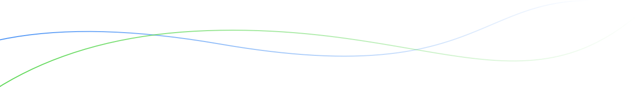
- Define the environments and groups and review the factors and variates.
- Environment Group (Mega-Environments): NONE
- Genotype: DESIGNATION
- Environment: SITE
- Select both variates; seed weight and 50% maturity.
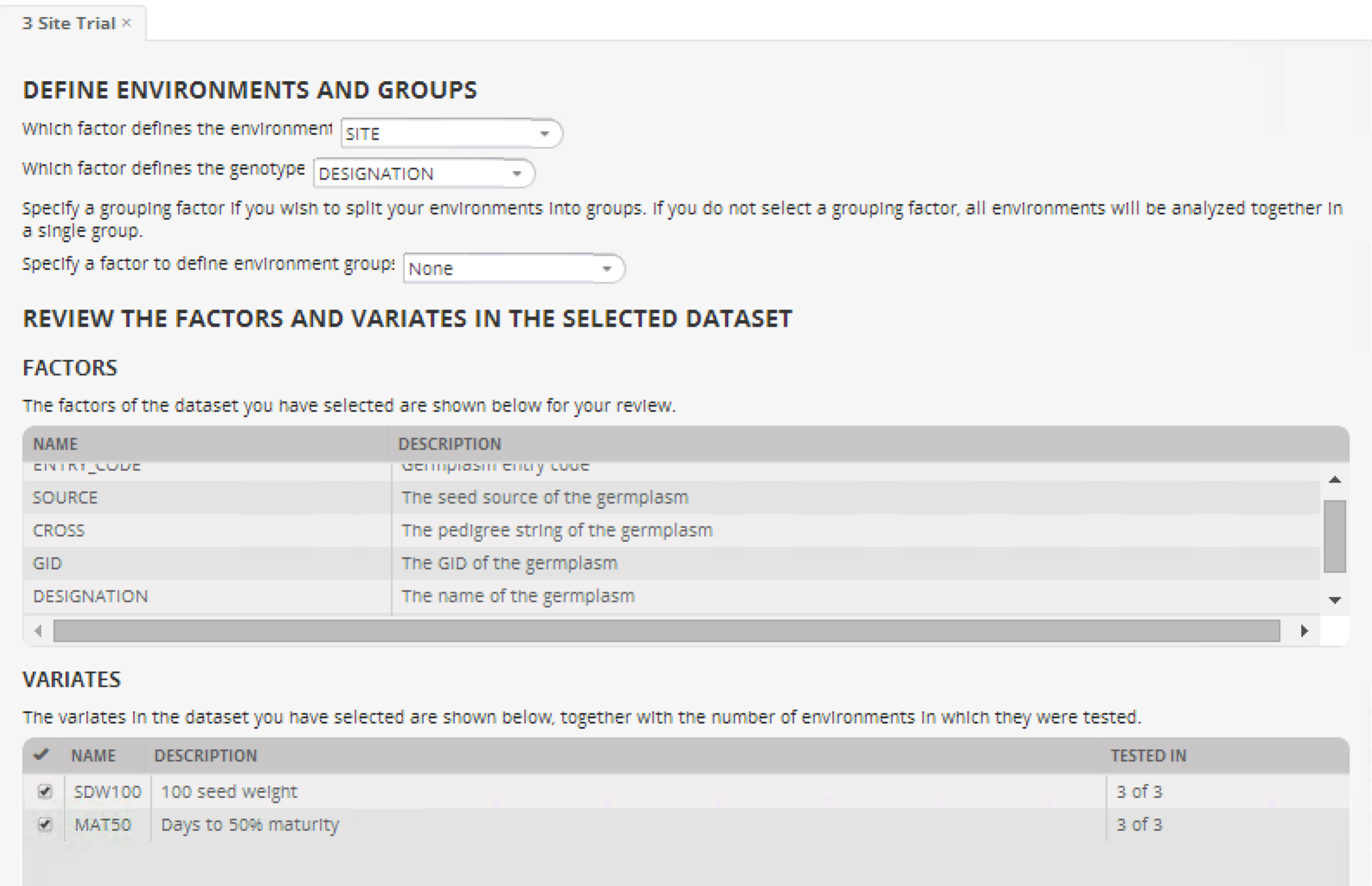
- Review the details of the dataset and launch Breeding View. Select Next.
Run Analysis
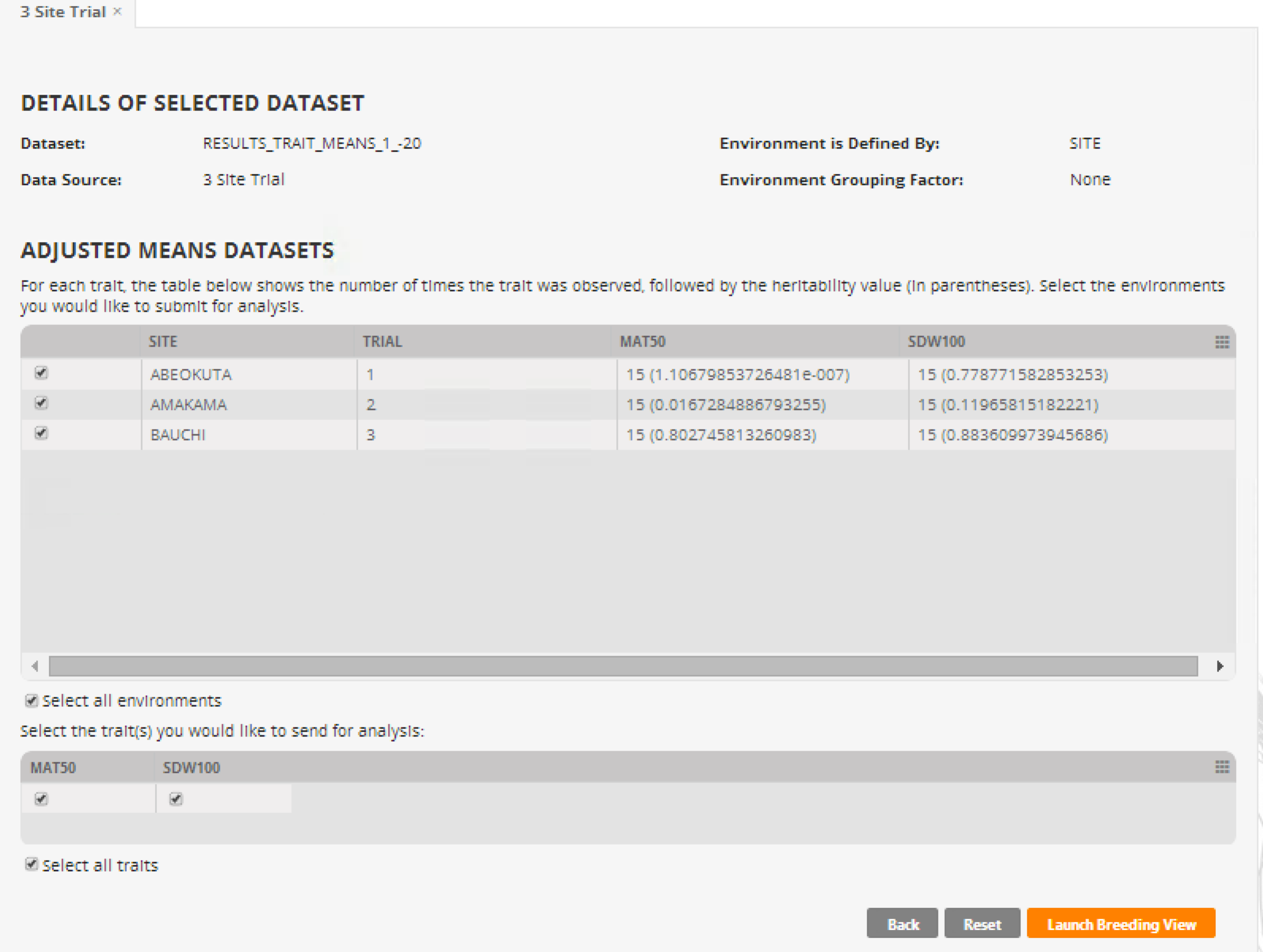
Mulit-Site analysis is database integrated. When the Breeding View application launches, the analysis conditions and data are automatically loaded. Notice that all locations and traits are selected by default. Right click on any trait or location to deselect from the analysis. When a project has been created or opened, a visual representation of the analytical pipeline is displayed in the Analysis Pipeline tab. The analysis pipeline includes a set of connected nodes, which can be used to run and configure pipelines.
- Right click on MAT50_Means and exclude this trait from the analysis.
Node Descriptions:
- Quality Control Phenotypes Summary statistics within and between environments for the trait(s)
- Finlay-Wilkinson: Performs a Finlay-Wilkinson joint regression
- AMMI Analysis:
- GGE Biplot
- Variance-Covariance Modeling: Selects the best covariance structure for genetic correlations between environments
- Stability Coefficients: Estimates different stability coefficients to assess genotype performance and generate HTML report of the results
Analysis Options
Some of the nodes have options to control they way an analysis is performed and output that is displayed. To access the options, right-click on a node and select the Settings item from the shortcut menu. Changes to the options are retained during the current session and are saved to the project file.
- Leave the default analysis settings. Right click on Quality Control Phenotypes to run pipeline. When the analysis is complete a popup window will notify you that the results are ready to view. ?
Results
Analysis results can be found in the Output, Graphs, and Results tab. Results are also saved in the Breeding Management System’s workspace folder.
Analysis Results
- Summary statistics for seed weight within and between the environments
- Sensitivity Calculations: Finlay-Wilkinson Joint Regression, AMMI, GGE,
- Stability statistics: Different variance-covariance models.
Summary Statistics
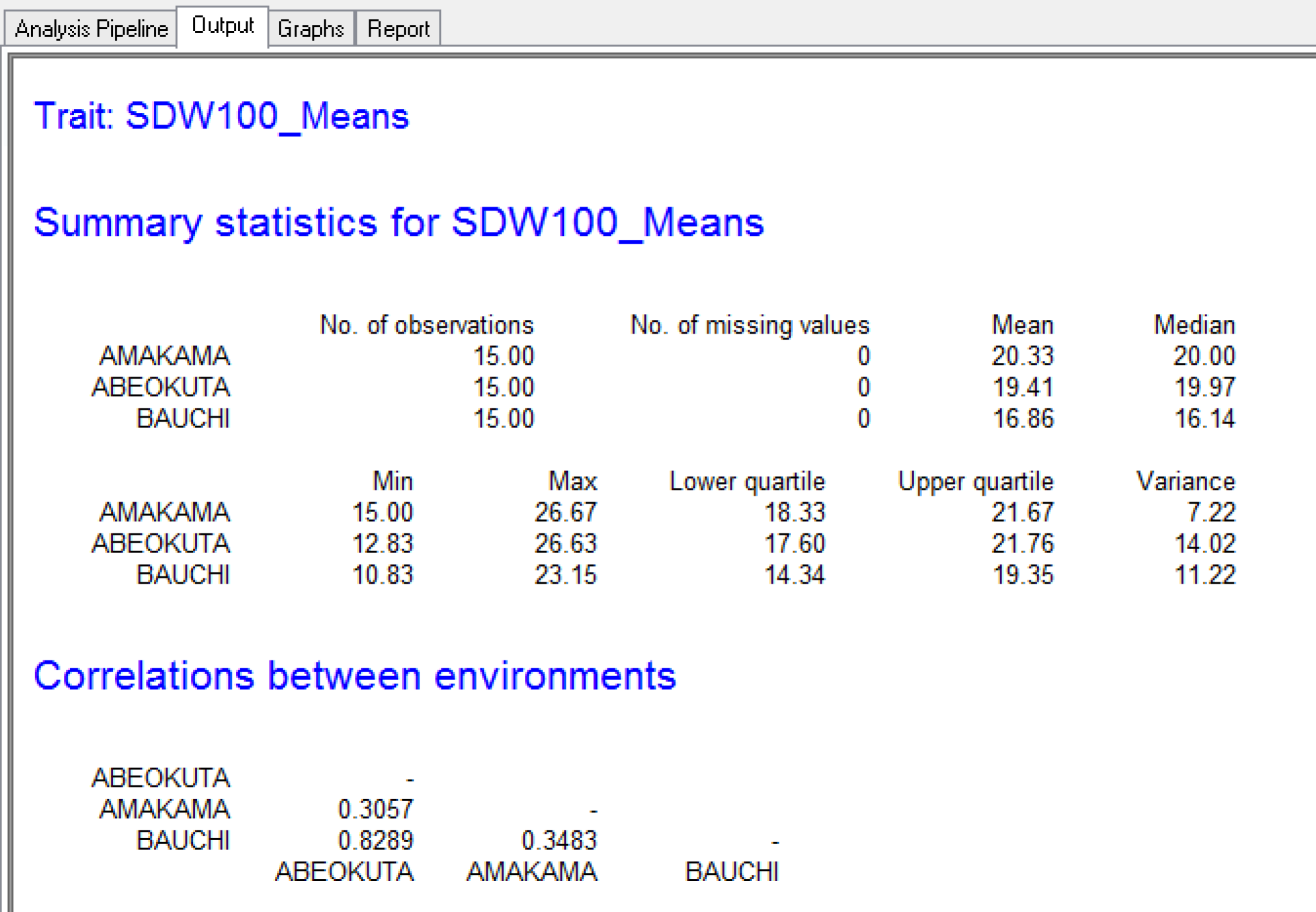 Summary statistics from the Output tab showing that the Amakama site has the highest mean seed weight and that the Abeokuta and Bauchi sites are highly correlated.
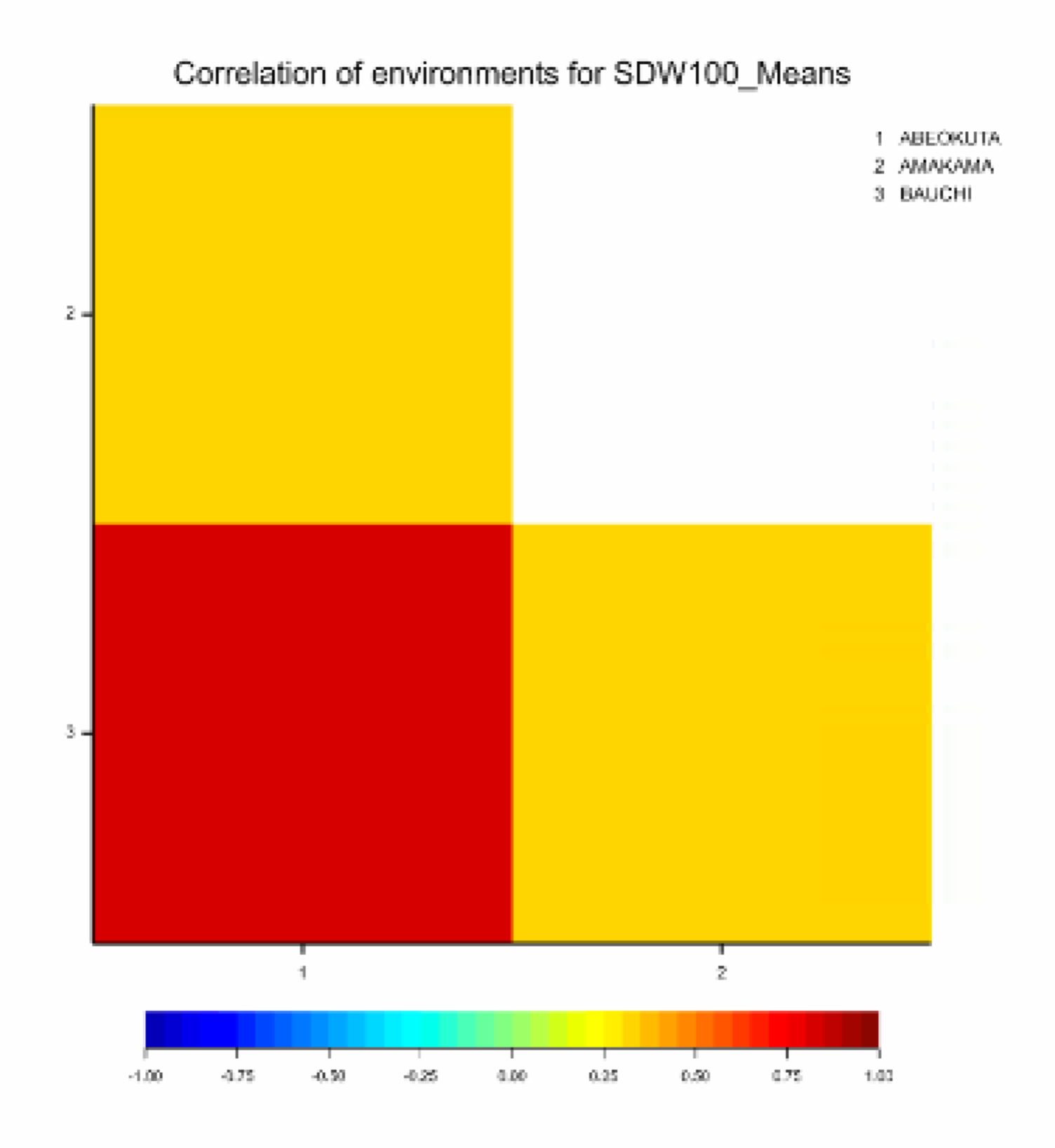
Graphical display of environmental correlations: The red coloration on the heat map indicates a high correlation (0.8289 from table in Output) between Abeokuta and Bauchi, and small correlations for the other two sites.
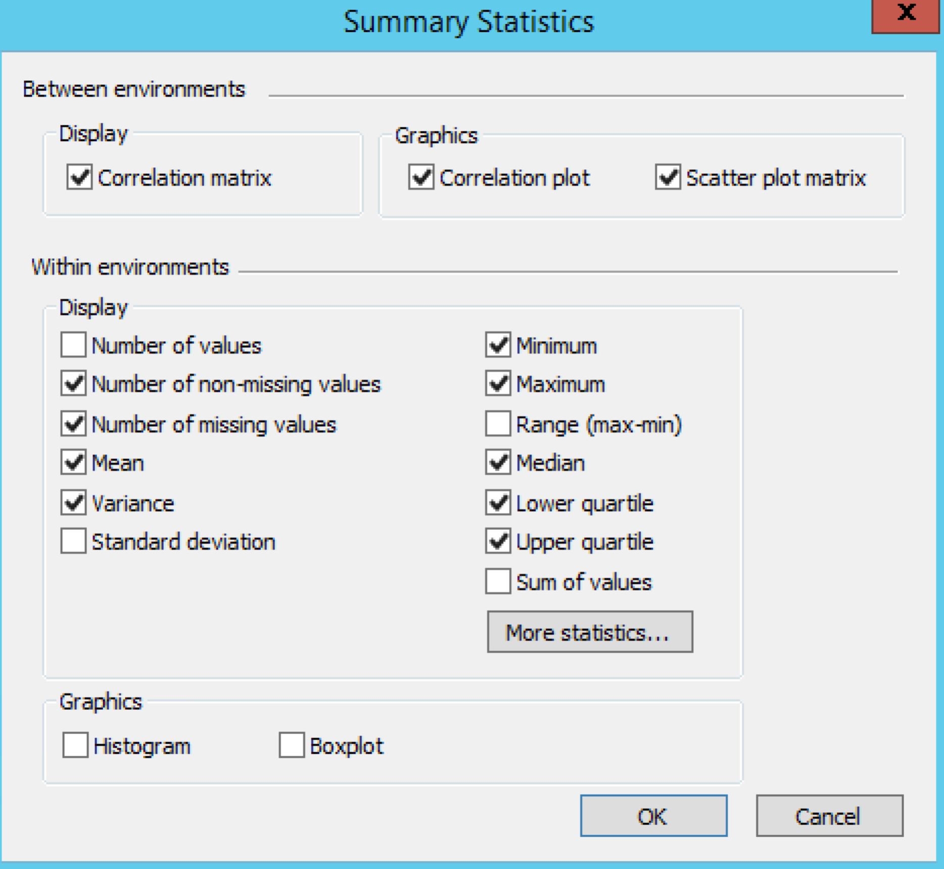
Default summary statistics options
Finlay-Wilkinson Joint Regression
Finlay-Wilkinson Joint Regression characterizes the sensitivity of each genotype to environmental effects by fitting a regression of the environment means for each genotypes on the average environmental means. In the estimates a value of 1 represents the average sensitivity and genotypes with a value greater than one exhibit higher than average sensitivity and genotypes with a value less than 1 are less sensitive than average.
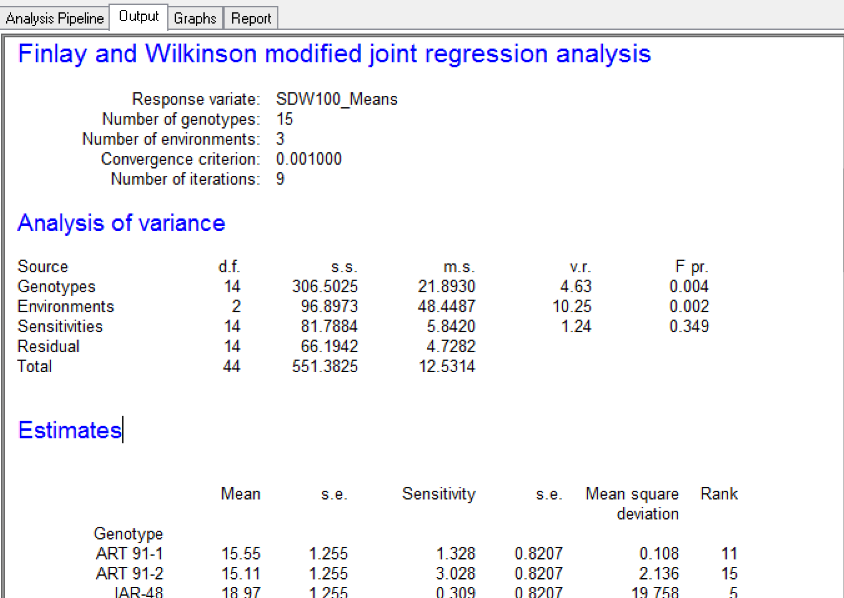
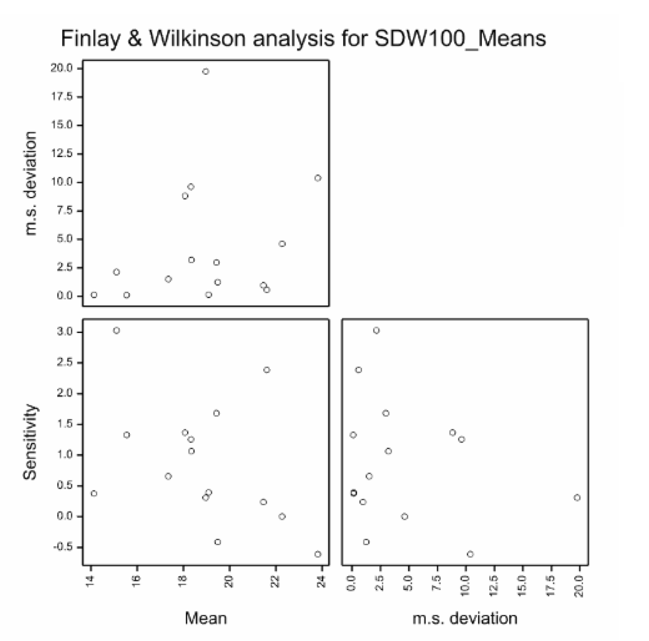
The Finlay Wilkinson analysis indicates that genotypes and environments are significant sources of variation (p = 0.004 and 0.002 respectively), but that G x E sensitivity is not significant (p=0.349). The most sensitive genotype is ART 91-2.
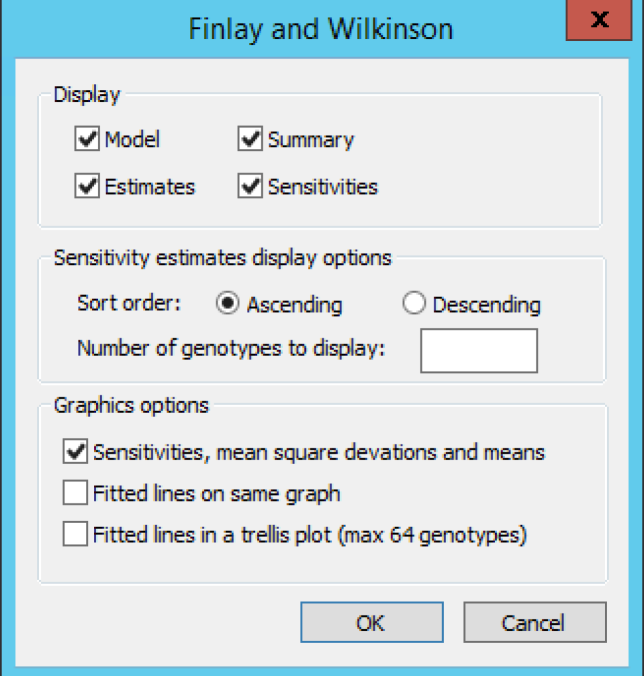
Default Finlay & Wilkinson options
AMMI Analysis
The AMMI analysis node fits a model which involves the Additive Main effects of ANOVA with the Multiplicative Interaction effects of principal components analysis (PCA). The AMMI model is more flexible than Finlay-Wilkinson, in that more than one environmental quality variable is explained using multiplicative terms.
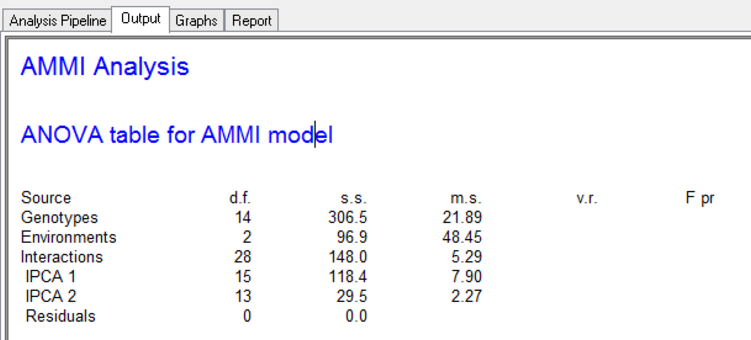
The ANOVA table for the AMMI analysis cannot be completed with variance and P values, because degrees freedom is limited by too few environments.
A desirable property of the AMMI model is that genotype and environmental scores can be used to construct biplots to help interpret genotype-by-environment interaction. In the biplot, genotypes that are similar to each other are closer in the plot than genotypes that are different. Similarly, environments that are similar will group together as well. When environment scores are connected to the origin of the plot, an acute angle between lines indicate a positive correlation between environments. A right angle between lines indicates low or no correlation between environments, and an obtuse angle indicates negative correlation. The projection of a genotype onto the environmental axis reflects performance in that particular environment.
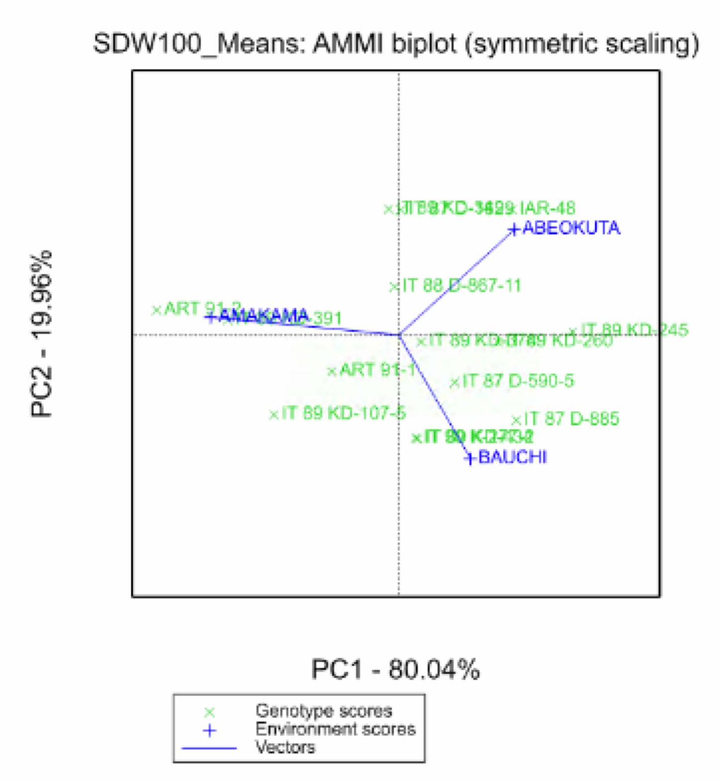
The obtuse angle between Amakama and both Bauchi and Abeokuta, indicate that Amakama is negatively correlated to the other two environments. The acute angle between Abeokuta and Bauchi reiterates the summary statistics result, that phenotypic responses at these two locations are correlated.
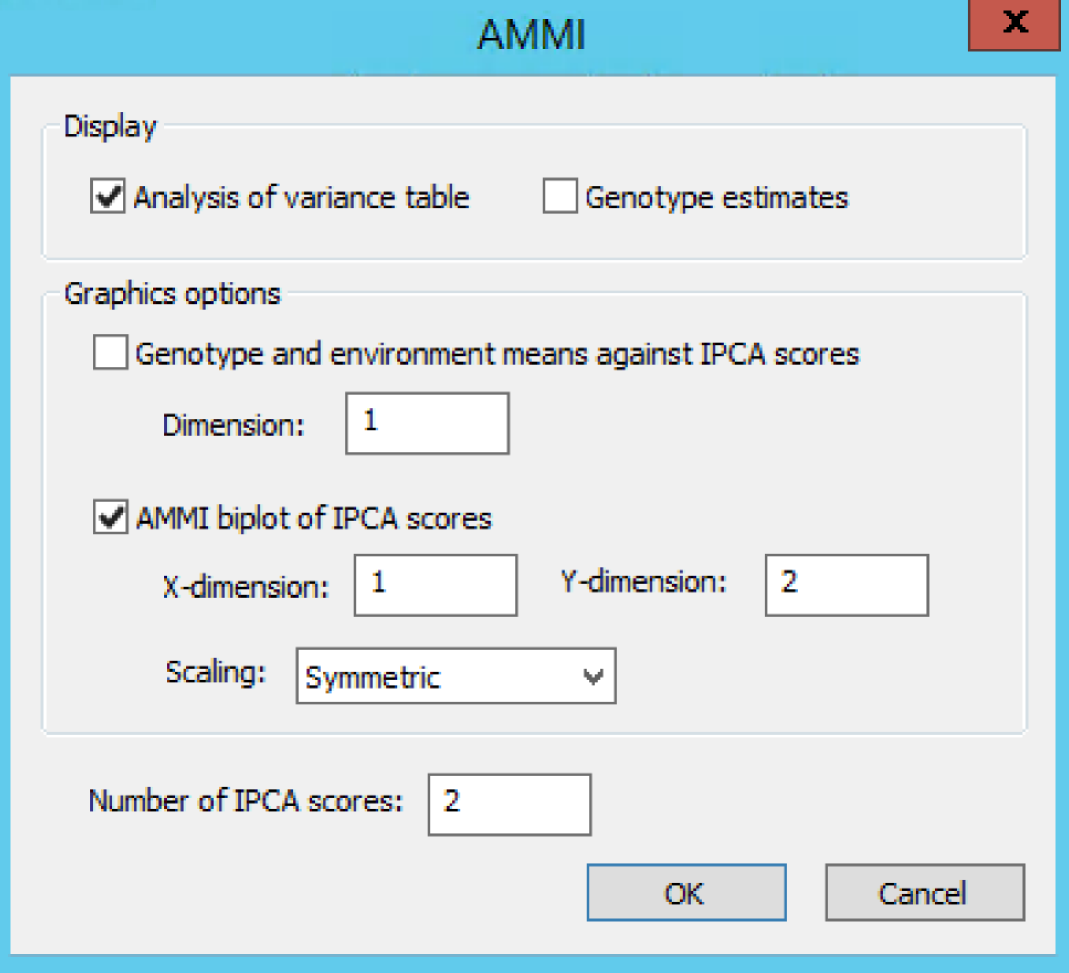
Default AMMI Analysis options
GGE Biplot
The GGE (genotype main effect (G) plus genotype-by-environment (GE) interaction) biplot is a modification of the AMMI model, which joins the effects of the genotypic main effects and the genotype-by-environment interaction (Yan & Kang, 2003). As this describes both the genotypic main effects and genotype-by-environment interaction together, it is known as a GGE model, and the biplots are called GGE biplots. The interpretation of the GGE biplot is similar to the AMMI biplot, but now the genotypes are distributed according to overall performance in each environment, rather than just genotype-by-environment interaction. In the GGE biplot, the best performing genotypes are on the right-hand side of the plot.
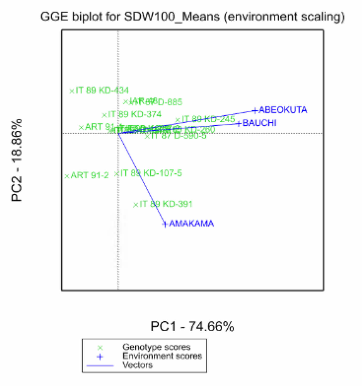
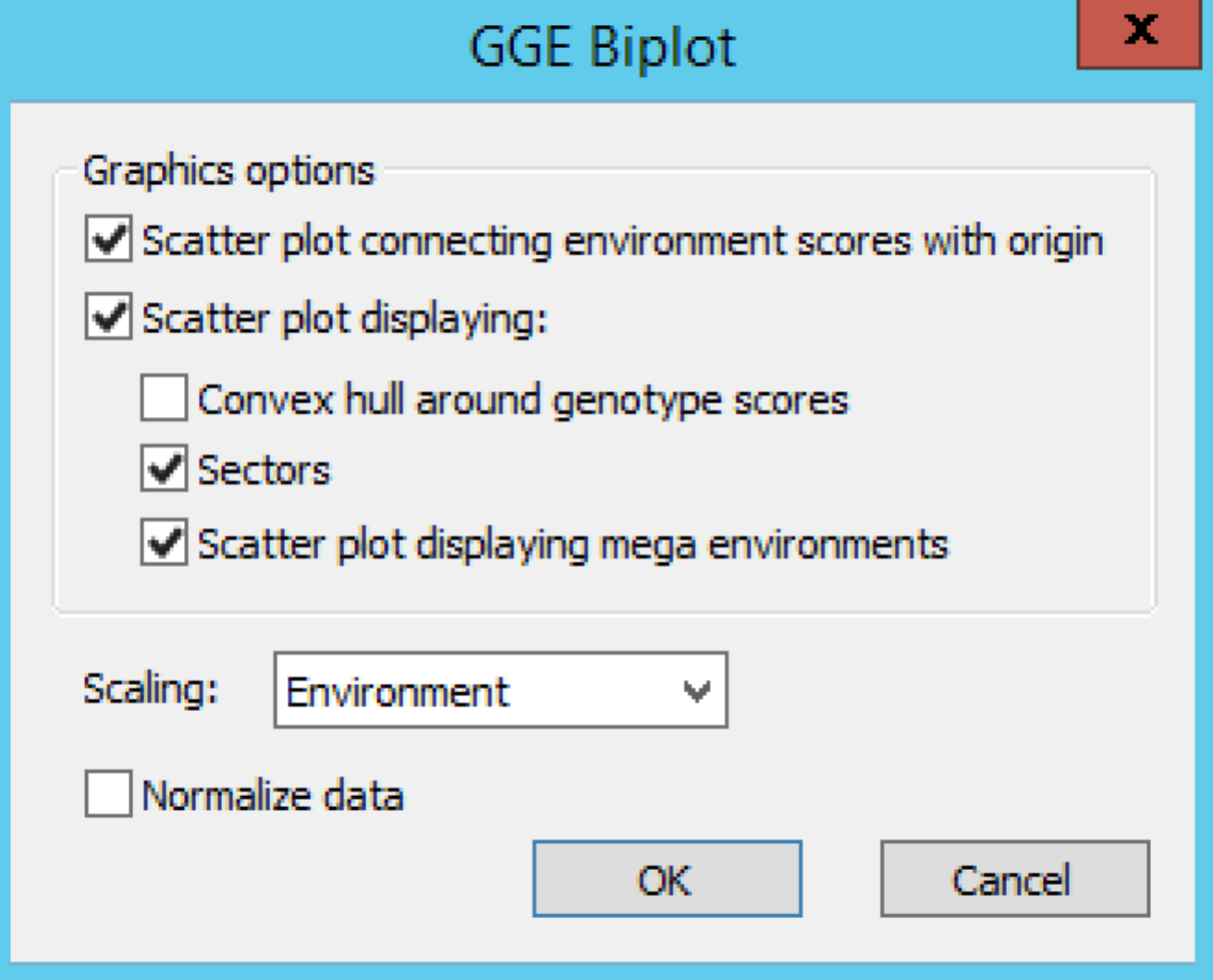
Default GGE Biplot options
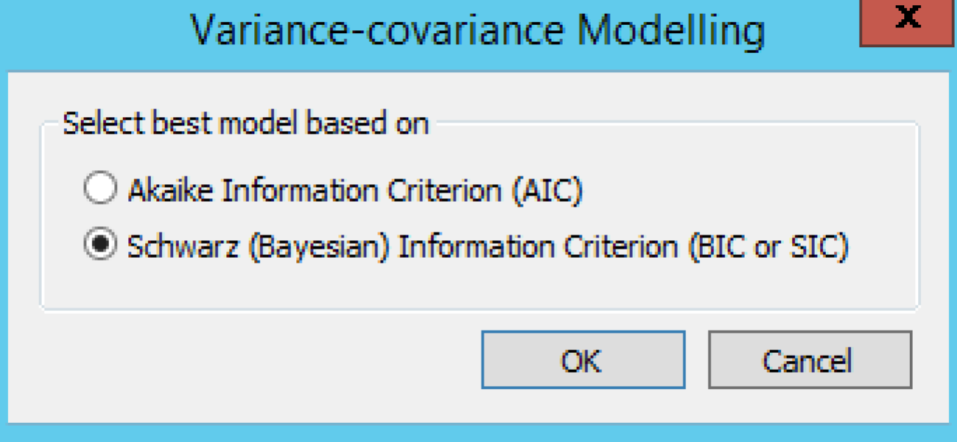
Variance-Covariance Modeling
Variance-covariance modeling is a mixed model approach to examination of genotype-by-environment interactions in terms of heterogeneity of variances and covariances. Breeding View evaluates a range of possible variance-covariance models and selects the best based on an information criterion.
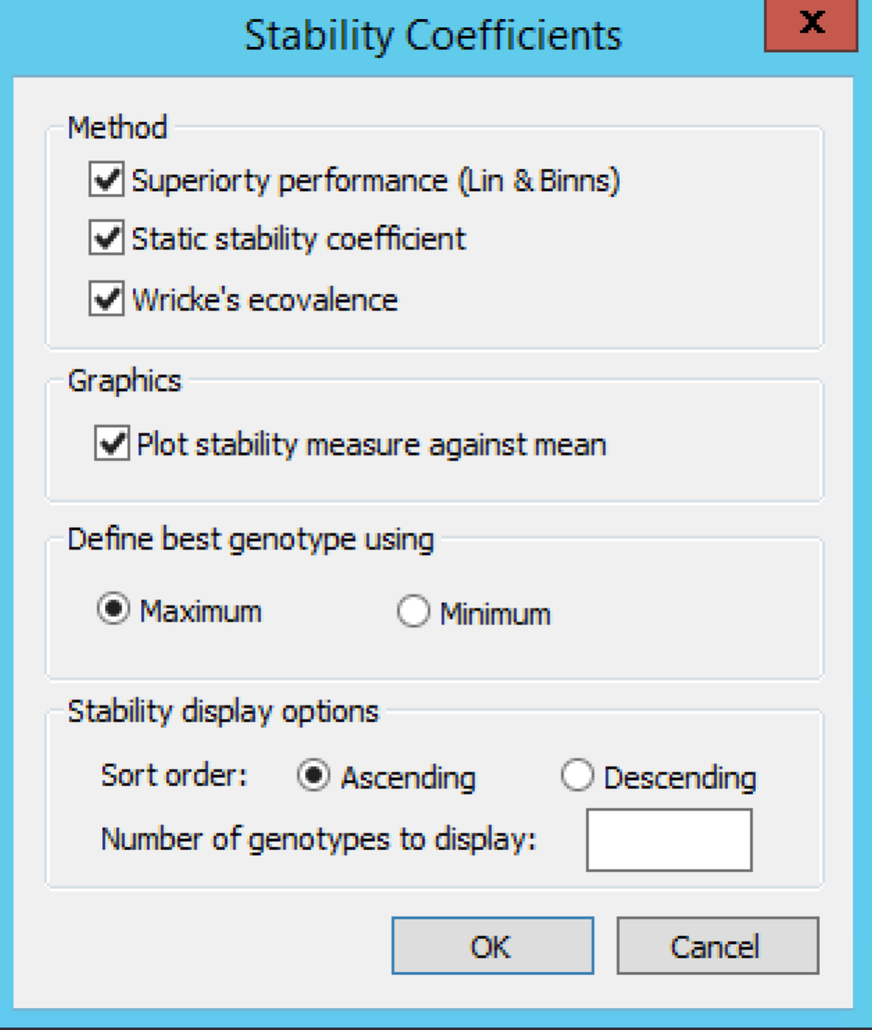
Stability coefficient measures for the genotypes:
- Cultivar-Superiority Measure (Lin & Binns, 1988): The sum of the squares of the difference between genotypic mean in each environment and the mean of the best genotype, divided by twice the number of environments. Genotypes with the smallest values of the superiority tend to be more stable, and closer to the best genotype in each environment.
- Static Stability Coefficient is defined as the variance between its mean in the various environments. This provides a measure of the consistency of the genotype, without accounting performance
- Wricke’s Ecovalence Stability Coefficient (Wricke, 1962): The contribution of each genotype to the genotype-by-environment sum of squares, in an un-weighted analysis of the genotype-by-environment means. A low value indicates that the genotype responds in a consistent manner to changes in environment.
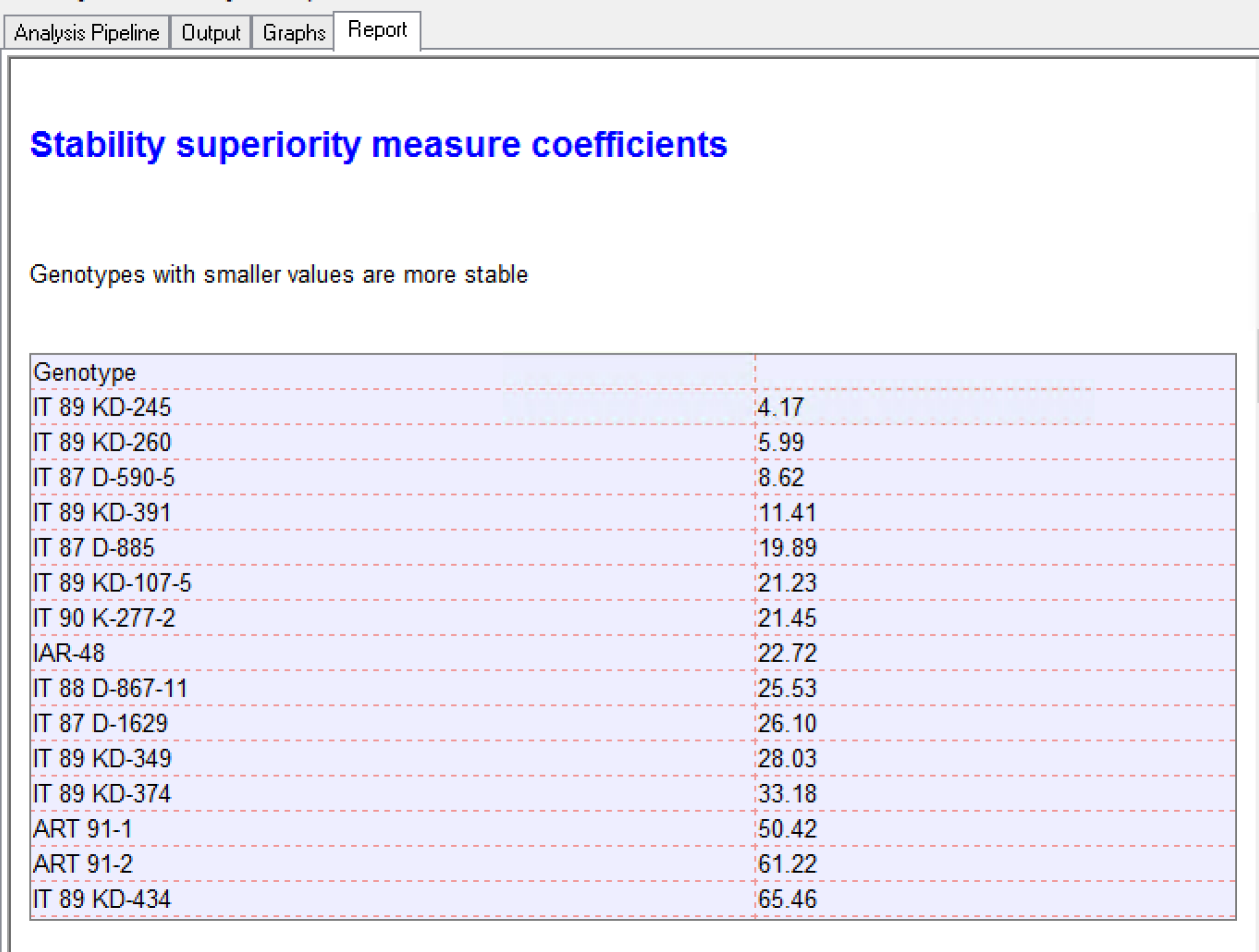 ?The most stable genotype identified by the Cultivar-Superiority Measure is IT 89-KD-245.
When Breeding View is run, the data files are automatically saved to your computer in the Workspace folder.
References
Cullis BR, Smith AB, Coombes NE (2006) On the design of early generation variety trials with correlated data. Journal of Agricultural Biological and Environmental Statistics 11(4), 381-393.
Gauch, H.G. (1992). Statistical Analysis of Regional Yield Trials – AMMI analysis of factorial designs. Elsevier, Amsterdam.
Finlay, K.W. & Wilkinson, G.N. (1963). The analysis of adaptation in a plant-breeding programme. Australian Journal of Agricultural Research, 14, 742-754.
Murray, D. Payne, R, & Zhang, Z. (2014) Breeding View, a Visual Tool for Running Analytical Pipelines: User Guide. VSN International Ltd. (.pdf) (Sample data .zip).
Lin, C.S. & Binns. M.R. (1988). A superiority performance measure of cultivar performance for cultivar x location data. Canadian Journal of Plant Science, 68, 193-198.
Wricke, G. (1962). Uber eine method zur erfassung der okogischen streubreite in feldversuchen. Zeitschriff Fur Pflanzenzuchtung, 47, 92-96.
Yan, W. & Kang, M.S. (2003). GGE Biplot Analysis: a Graphical Tool for Breeders, Geneticists and Agronomists. CRC Press, Boca Raton.
Funding & Acknowledgements
The Integrated Breeding Platform (IBP) is jointly funded by: the Bill and Melinda Gates Foundation, the European Commission, United Kingdom's Department for International Development, CGIAR, the Swiss Agency for Development and Cooperation, and the CGIAR Fund Council. Coordinated by the Generation Challenge Program the Integrated Breeding Platform represents a diverse group of partners; including CGIAR Centers, national agricultural research institutes, and universities.
The statistical algorithms in the Breeding View were developed by VSN International Ltd in collaboration with the Biometris group at University of Wageningen. Cowpea ?demonstration data was provided by Jeff Ehlers, Tim Close, Philip Roberts, Bao Lam Huyuh at the University of California Riverside and Issa Drabo at the Institut de l'Environnement et de Recherches Agricoles in Burkina Faso. These data may have been adapted for training purposes. Any misrepresentation of the raw breeding data is the solely the responsibility of the IBP.

This work is licensed under a Creative Commons Attribution-ShareAlike 4.0 International License.?
