Summary
This tutorial describes a genotype by environment (GxE) analysis for a four location maize field trial. This tutorial builds upon the adjusted means (BLUEs) and summary statistics calculated for the individual locations in the previous tutorial, Single Site Analysis: 4 Location Batch.
- Select Data from Database
- Generate BV Input Files from BMS
- Load Project & Data
- Run Analysis
- Analysis Report & Graphs
- References
- Related Materials
Select Data from Database
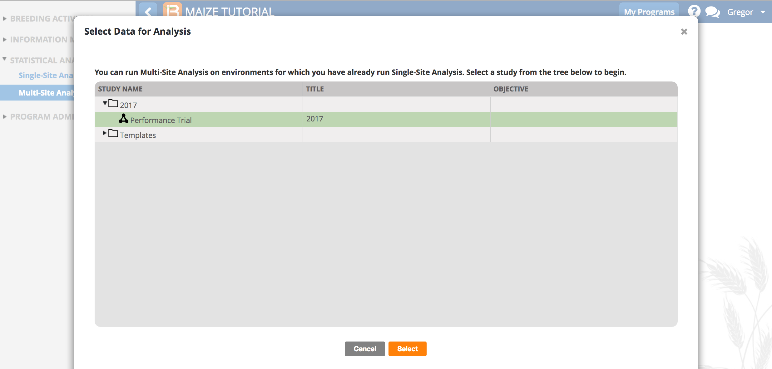
- Open Multi-Site Analysis from the Statistical Analysis menu of the Workbench. Select Browse.

- Select Performance Trial to use the BLUEs and summary statistics uploaded to the BMS after the single site analysis.
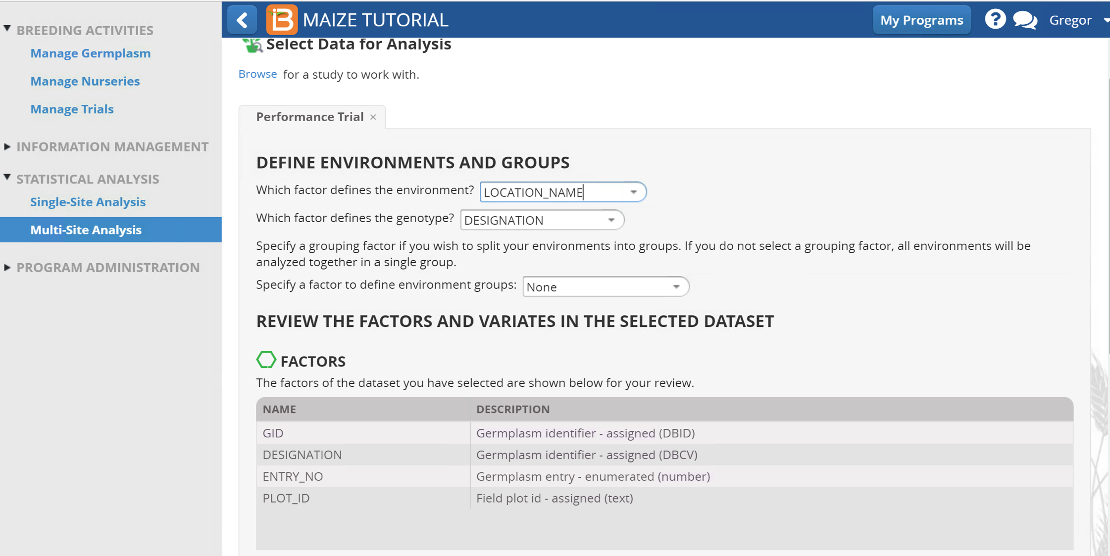
- Define environments and groups.
- Environments: LOCATION_NAME
- Genotype: DESIGNATION
- Environment Grouping Factor: None
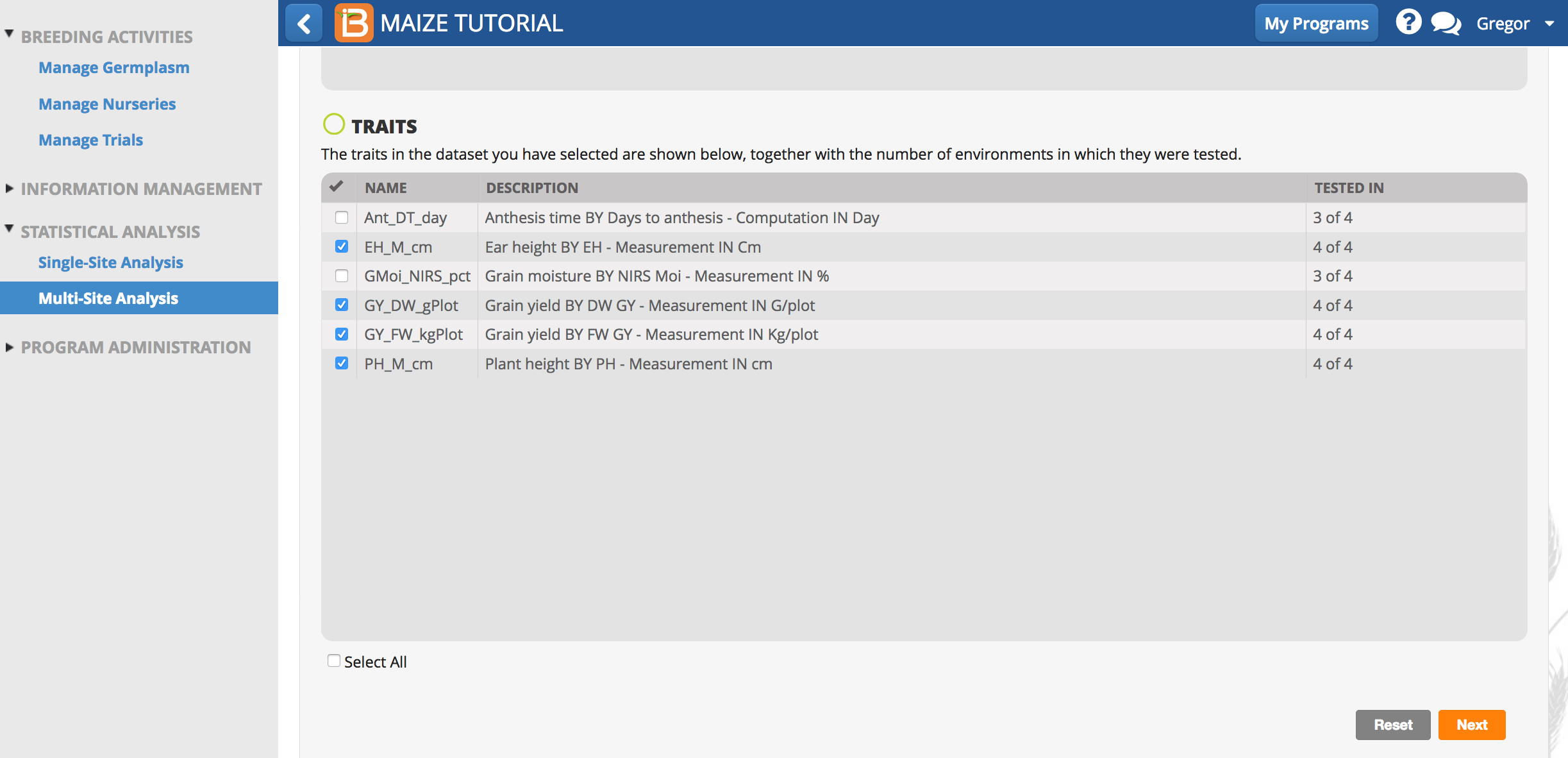
Traits with means available from all trial locations are selected by default. Traits that are not observed or could not be fitted with a mixed model in more than one environment in the single site analysis are not selected.
- Review the factors and variables in the dataset. Leave the default selections and select Next.
Generate BV Input Files from BMS
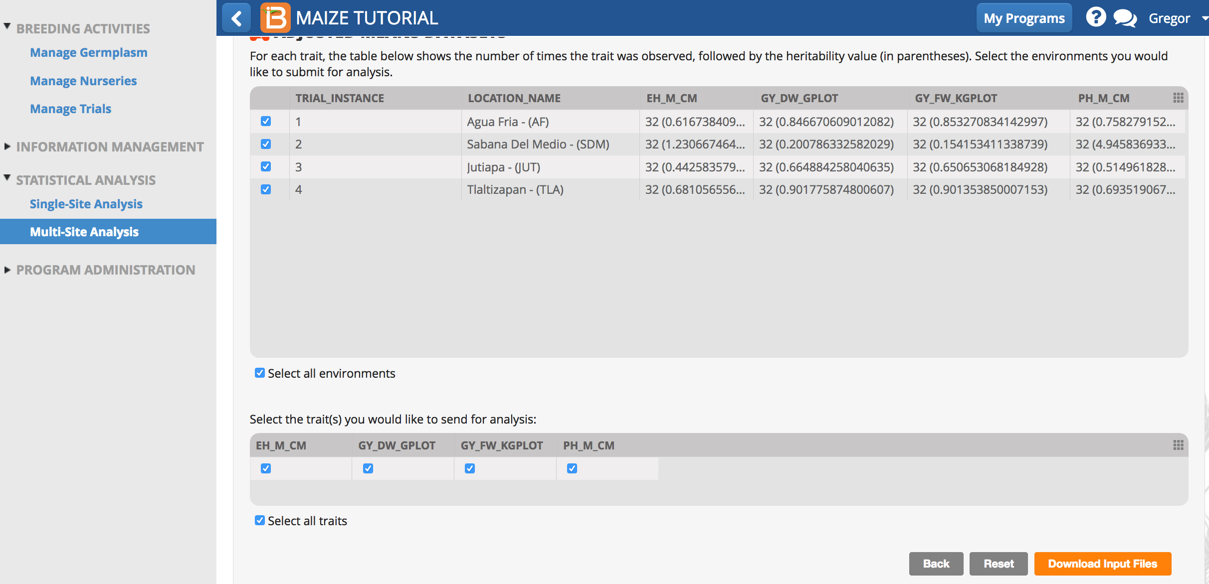
- Review the four environments and four traits to be included in the multi-site analysis. Select Download Input Files.
Load Project & Data
- The BV Input Files are located within a compressed folder automatically titled Performance Trial. The Breeding View .xml file is located within the Performance Trial folder. Open BV application and select Open Project and browse to the .xml Breeding View project file. The .xml file will load the genotypic and environmental summary statistics.
Run Analysis
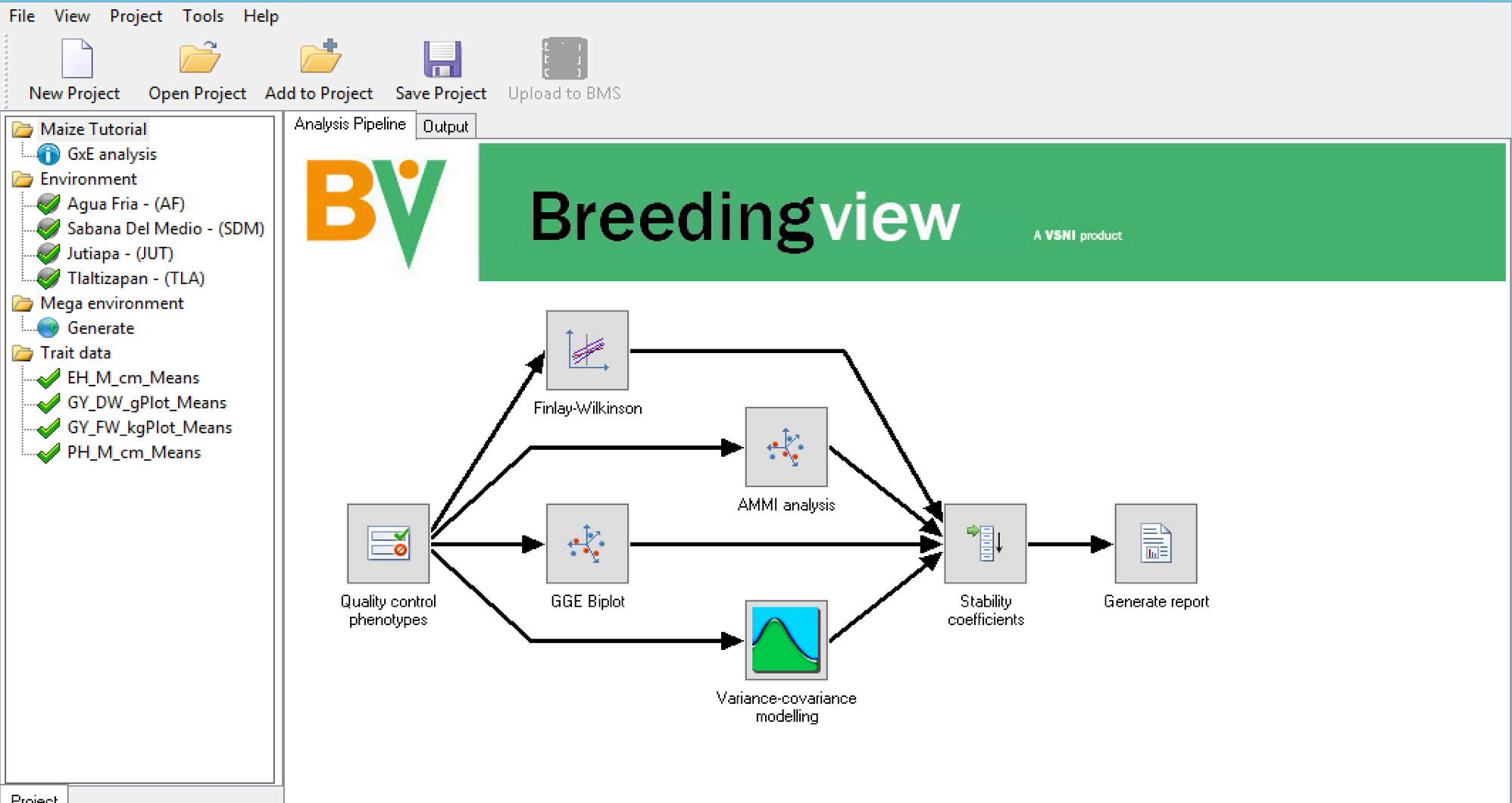
When a project has been created or opened, a visual representation of the analytical pipeline is displayed in the Analysis Pipeline tab. The analysis pipeline includes a set of connected nodes, which can be used to run and configure pipelines.
Node Descriptions:
- Quality Control Phenotypes: Summary statistics within and between environments for the trait(s)
- Finlay-Wilkinson: Performs a Finlay-Wilkinson joint regression (Finlay and Wilkinson, 1963)
- AMMI Analysis: Fits an AMMI model and generates summaries and a biplot (Gauch, 1988)
- GGE Biplot: Fits a GGE model and generates a biplot (Yan et al., 2000).
- Variance-Covariance Modeling: Fits different variance-covariance models to the GxE data and selects the best one for the data
- Stability Coefficients: Estimates different stability coefficient parameters to assess genotype performance
- Generate report: Generates an HTML report of the results
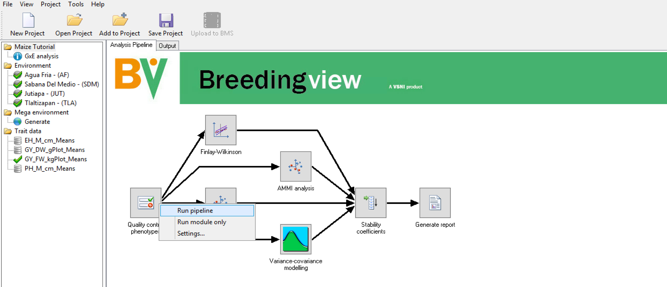
- Exclude all traits except grain yield t/ha (GY_FW_kgPlot_Means) from the analysis.
- Run the analysis using the default settings by right clicking the Quality Control Phenotype node and choosing Run Pipeline.
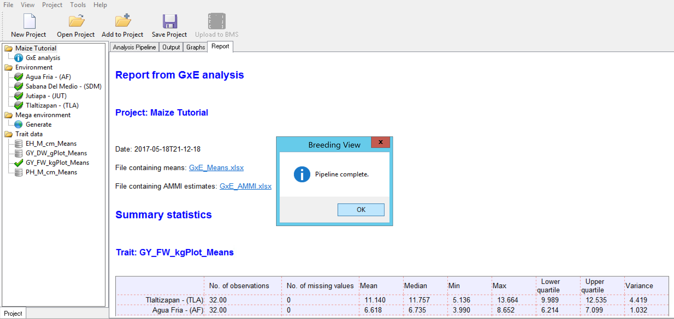
When the analysis is complete a popup notifies the user.
- Select OK.
Analysis Report & Graphs
The analysis output can be viewed from Breeding View interface under the results and graphs tabs. Analysis results can also be reviewed as individual files are automatically saved in the location specified by your browser settings, generally the Downloads folder..
Descriptive Statistics
Breeding View provides descriptive statistics that describe the variance and covariance of the entire dataset.
Trait Summary Statistics
The trait summary statistics describe each trait based on the means calculated for each environment in the single site analysis.

The box plot of means provides a visual representation of the summary statistics.
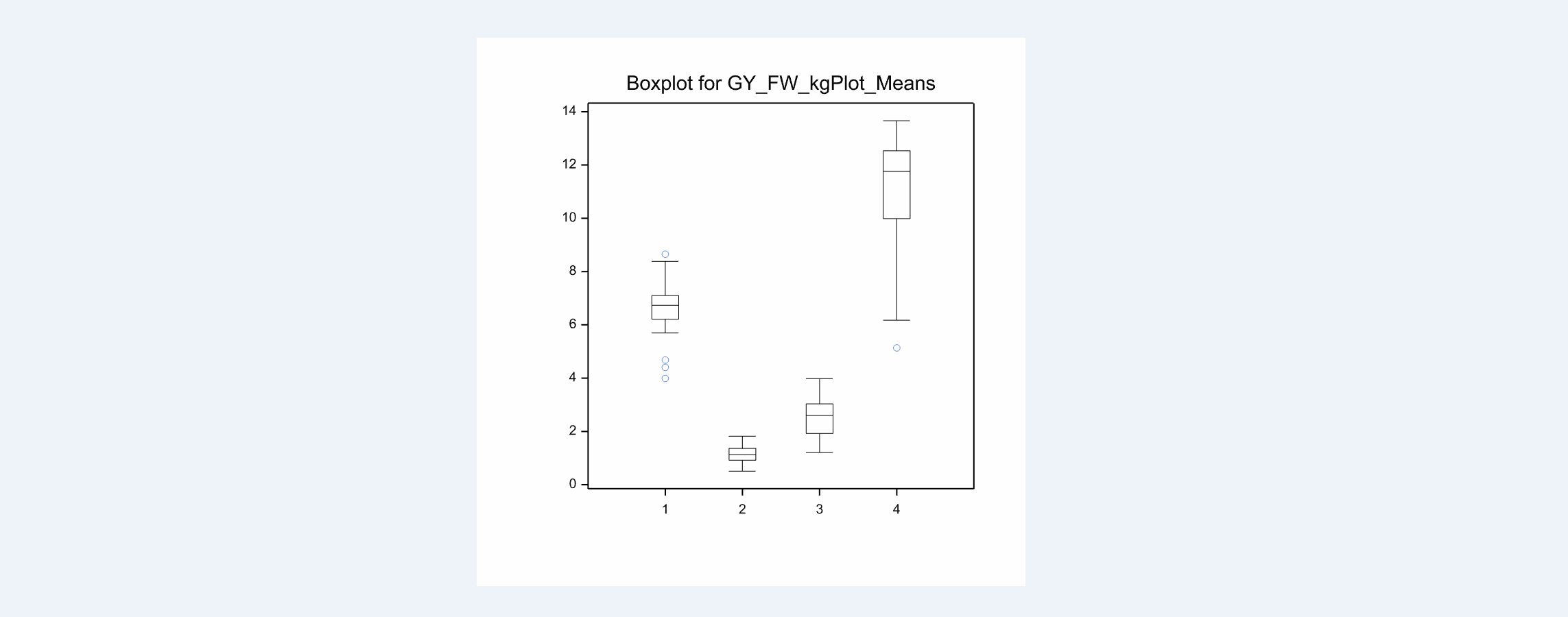
Boxplot of Grain Yield Means: Tlalzipan has the highest grain yield and the highest variance. Sabana Del Medio has the lowest grain yield and the lowest variance.
Best Variance-Covariance Model for Each Trait
The GxE analysis pipeline formally models the variance-covariance structure in the means data and selects the best model for each trait. The main purpose is to establish a model for later testing of fixed effects, like determining marker effects in a quantitative trait loci by environment (QTLxE) analysis using BLUPs calculated in the single site analysis.
 Best Variance-Covariance Model: In this example, grain yield means are best described by an unstructured model, where each variance and covariance is estimated uniquely from the data.?
Genotype By Environment (GxE) Interactions
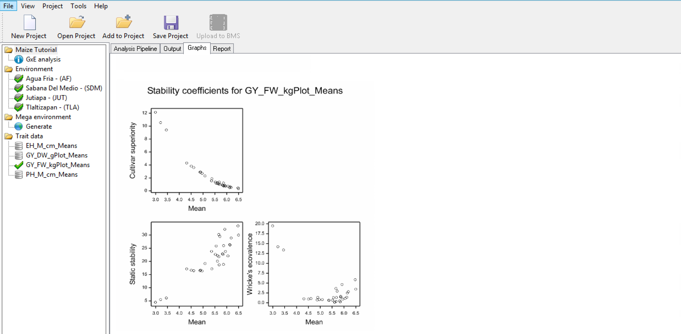
Stability, or lack of phenotypic plasticity, is calculated for each genotype considering all traits using the following analyses:
- Cultivar-Superiority Measure
- Static Stability Measures Coefficients
- Wricke’s Ecovalence Stability Coefficients
GxE interactions are also examined for each individual trait using the following analyses:
- Finlay and Wilkinson Modified Joint Regression
- AMMI Model
- GGE Model
- Best Variance-Covariance Model
- Correlation Matrix
- Scatter Plot Matrix
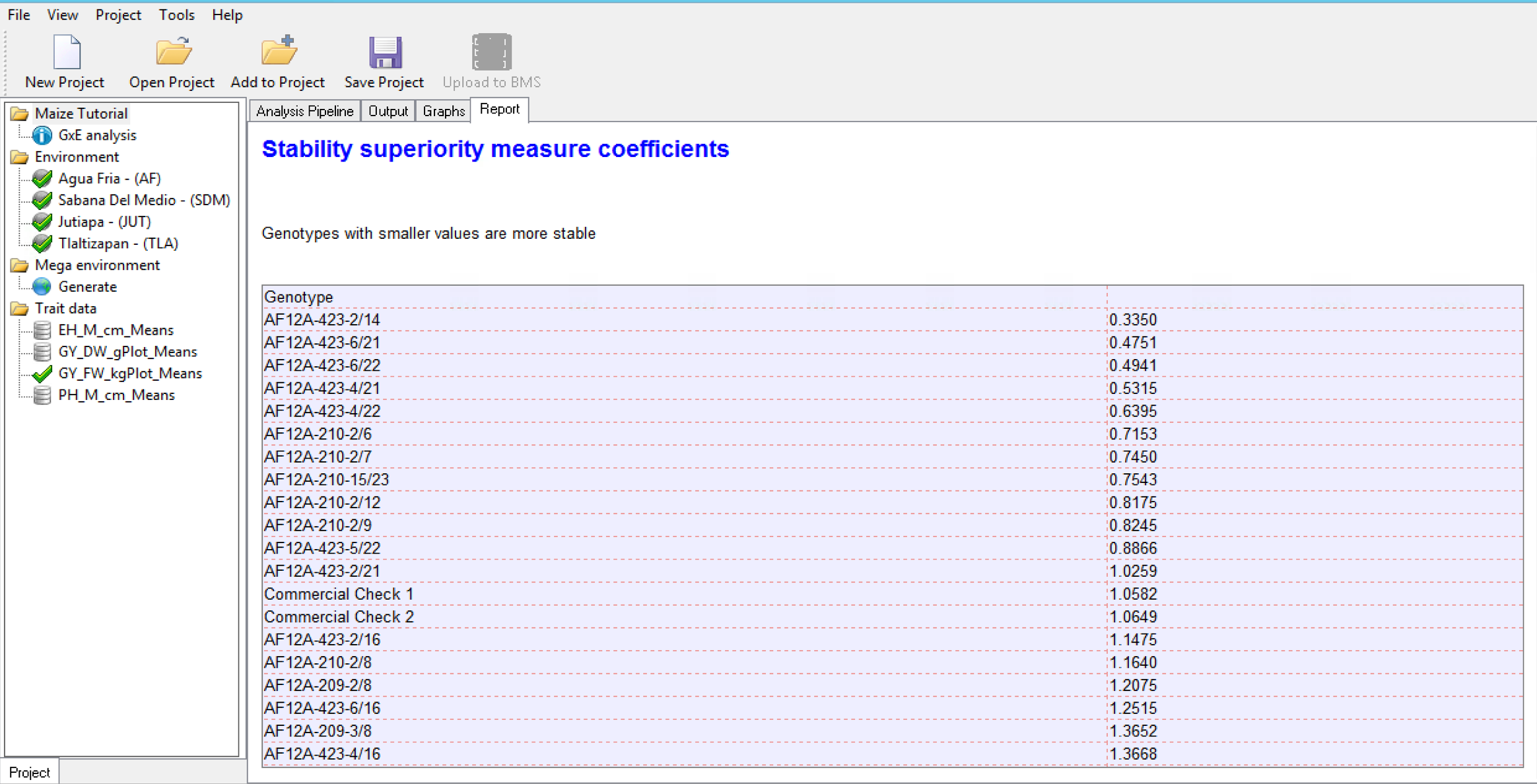
Stability Superiority Measure
Stability Superiority Measure (Lin & Binns,1988) is the sum of the squares of the difference between genotypic mean in each environment and the mean of the best genotype, divided by twice the number of environments. Genotypes with the smallest values of the superiority tend to be more stable, and closer to the best genotype in each environment.
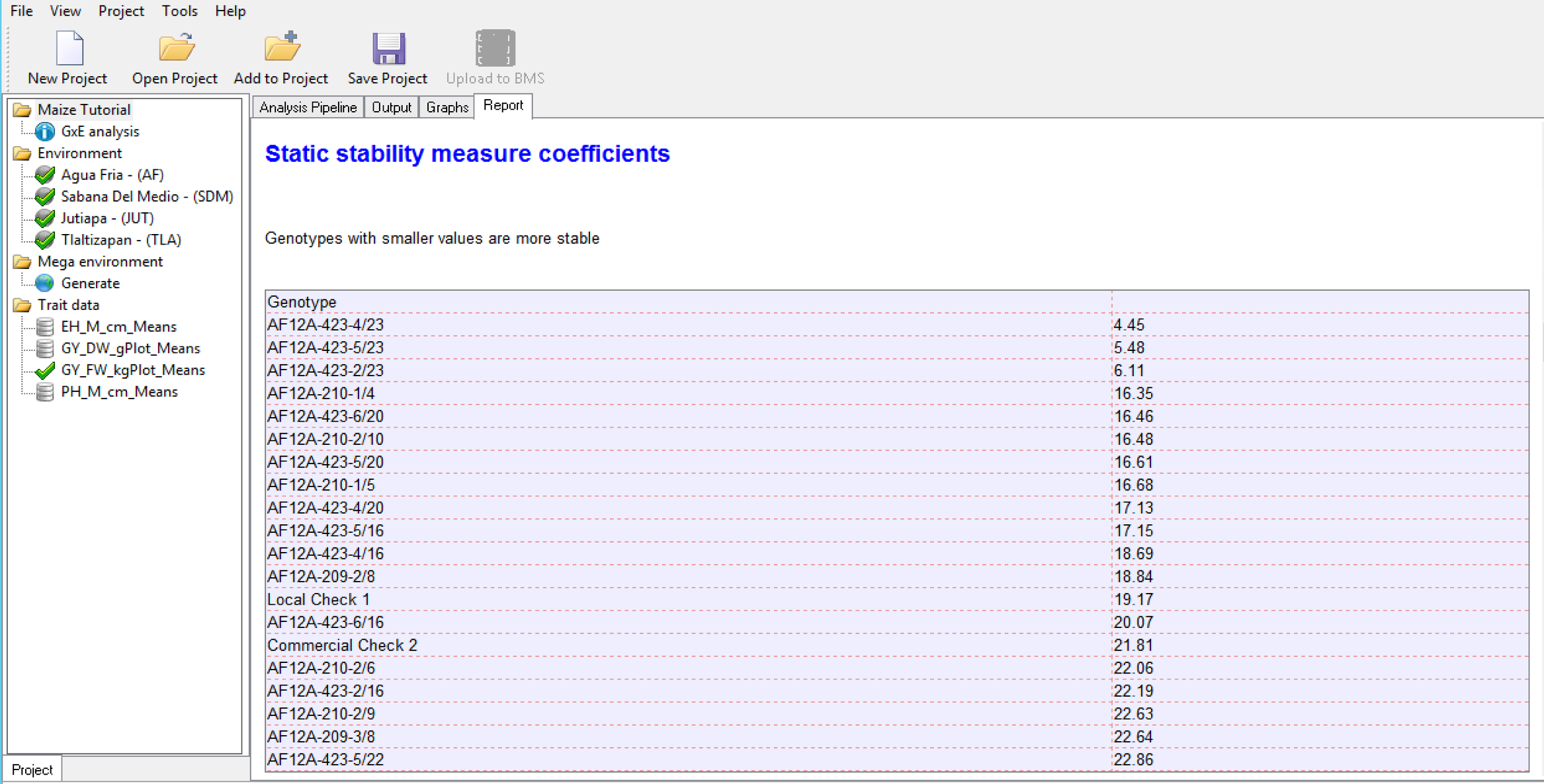
Static Stability Measures Coefficients
The Static Stability Coefficient is defined as the variance around the germplasm’s phenotypic mean across all environments. This provides a measure of the consistency of the genotype, without accounting for performance.
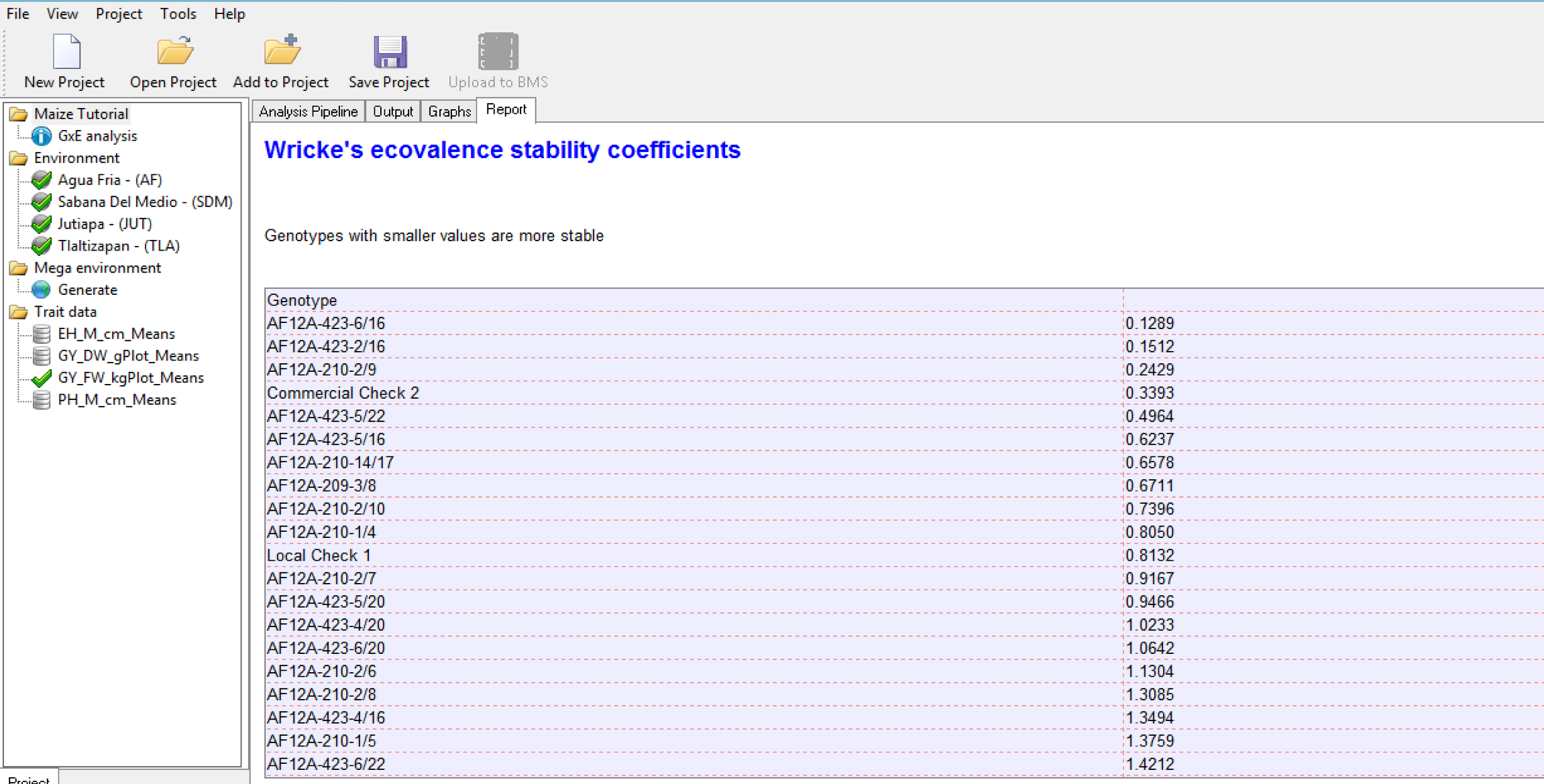
Wrick’s Ecovalence Stability Coefficients
Wricke’s Ecovalence Stability Coefficient (Wricke, 1962) is the contribution of each genotype to the genotype-by-environment sum of squares, in an un-weighted analysis of the genotype-by-environment means. A low value indicates that the genotype responds in a consistent manner to changes in environment; i.e. stable from a dynamic point of view. Like static stability, the Wricke’s Ecovalence does not account for genotype performance.
Finlay and Wilkinson Modified Joint Regression Analysis
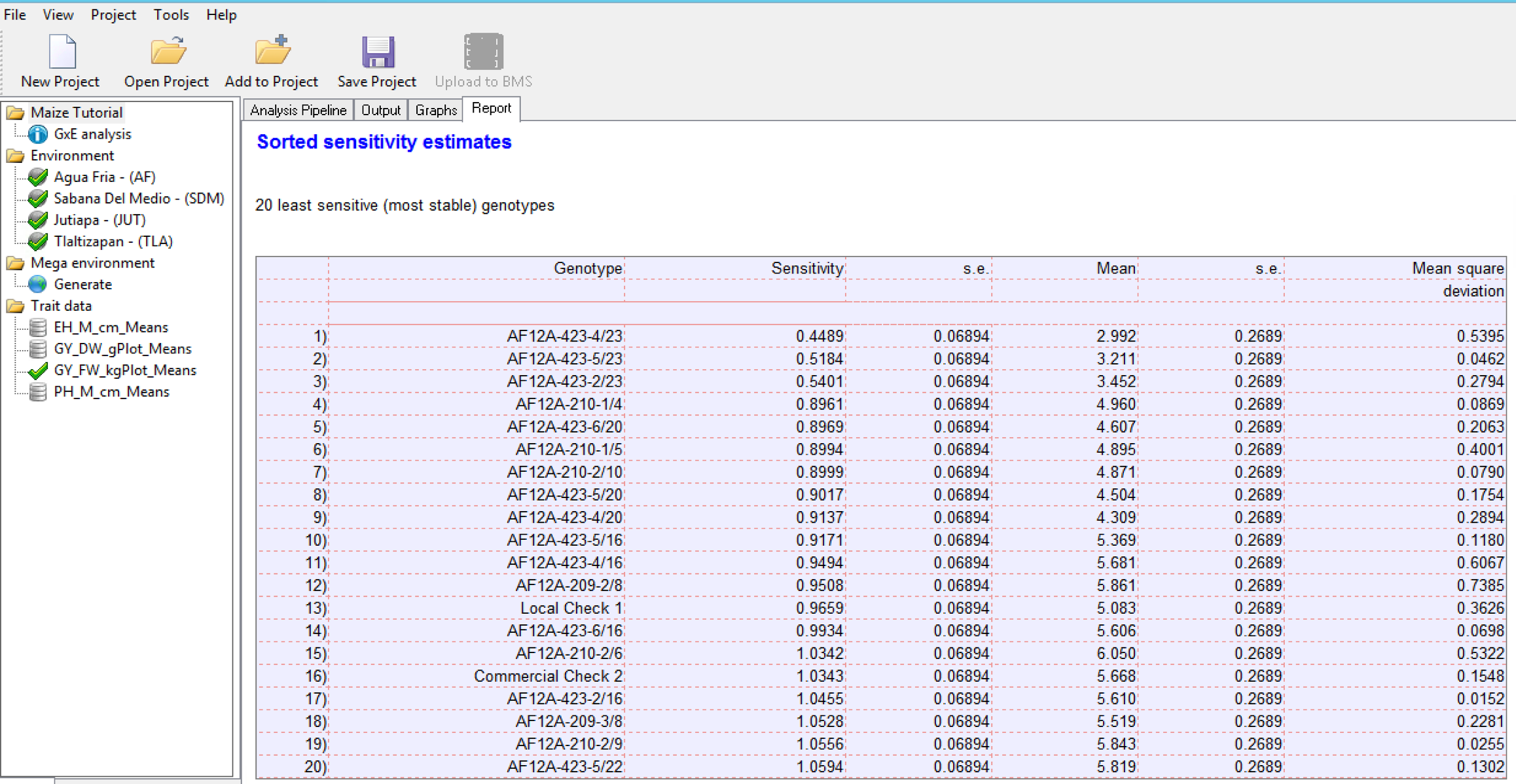
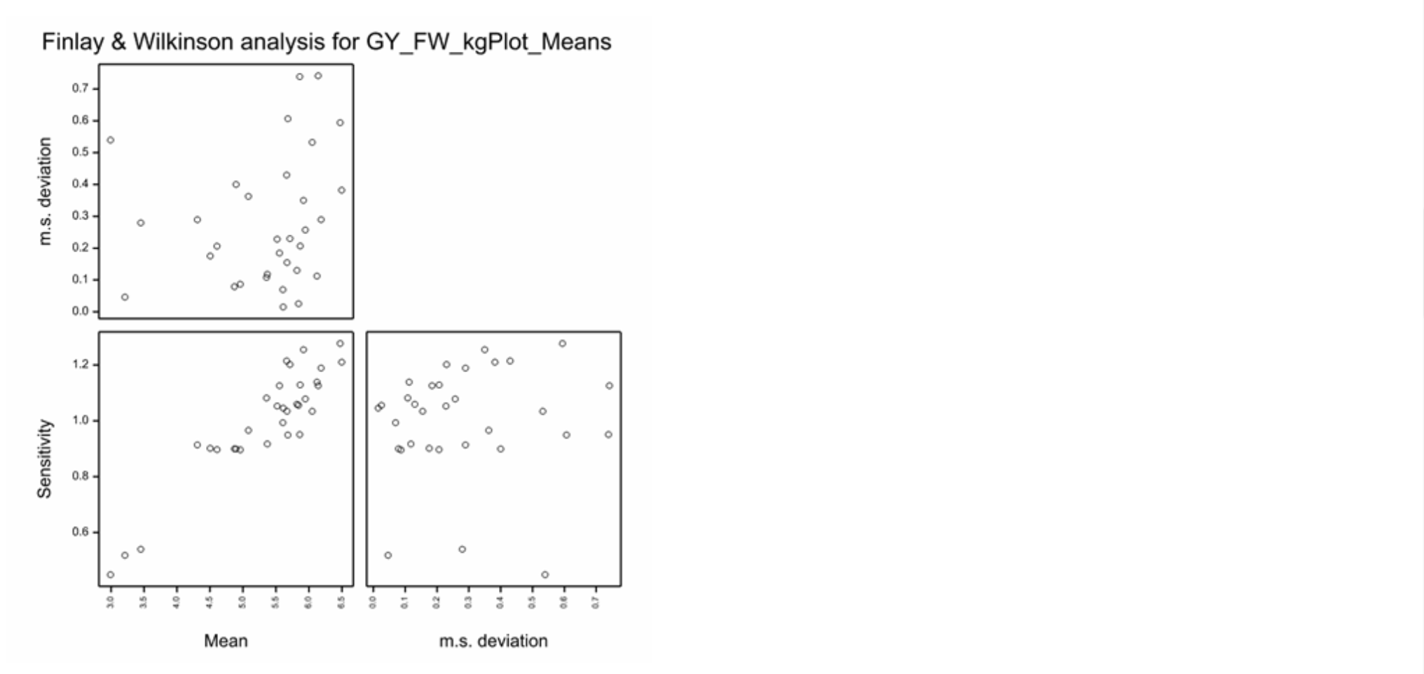
The Finlay and Wilkinson Modified Joint Regression Analysis ranks germplasm based on phenotypic stability for each individual trait.
AMMI Model
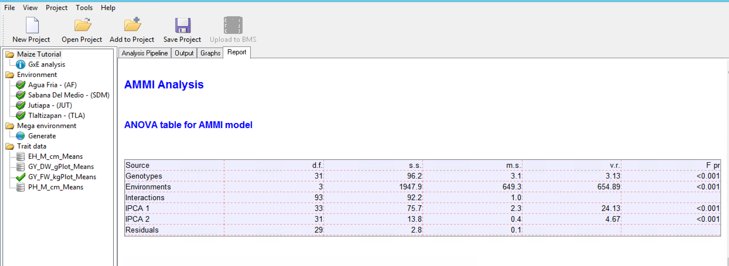
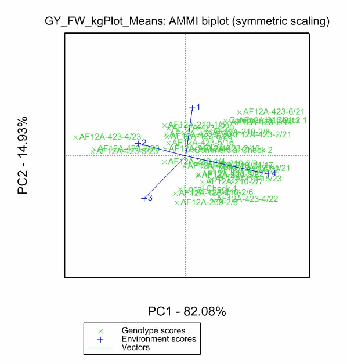
In the Additive Main Effects and Multiplicative Interaction (AMMI) model, a two-way ANOVA additive model is performed (additive main effects), followed by a principal component analysis on the residuals (multiplicative interaction). As a result, the interaction is characterized by Interaction Principal Components (IPCA), where genotypes and environments can be simultaneously plotted in biplots.
GGE Model
In the Genotype Main Effects and Genotype × Environment Interaction Effects (GGE) model (Yan et al. 2000 & 2003) a 1-way ANOVA, including environment as a main effect, is run followed by a principal component analysis on the residuals. Like AMMI, principal component scores can be used to construct biplots. Unlike the AMMI Model, in GGE the genotypic main effects are also represented in the plot. The GGE model is superior to AMMI analysis at differentiating mega-environments (Yan et al. 2007)
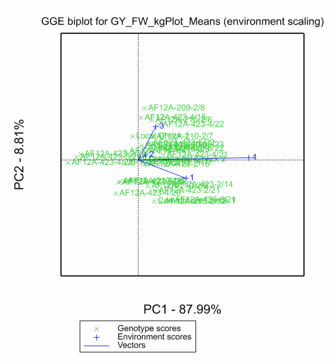
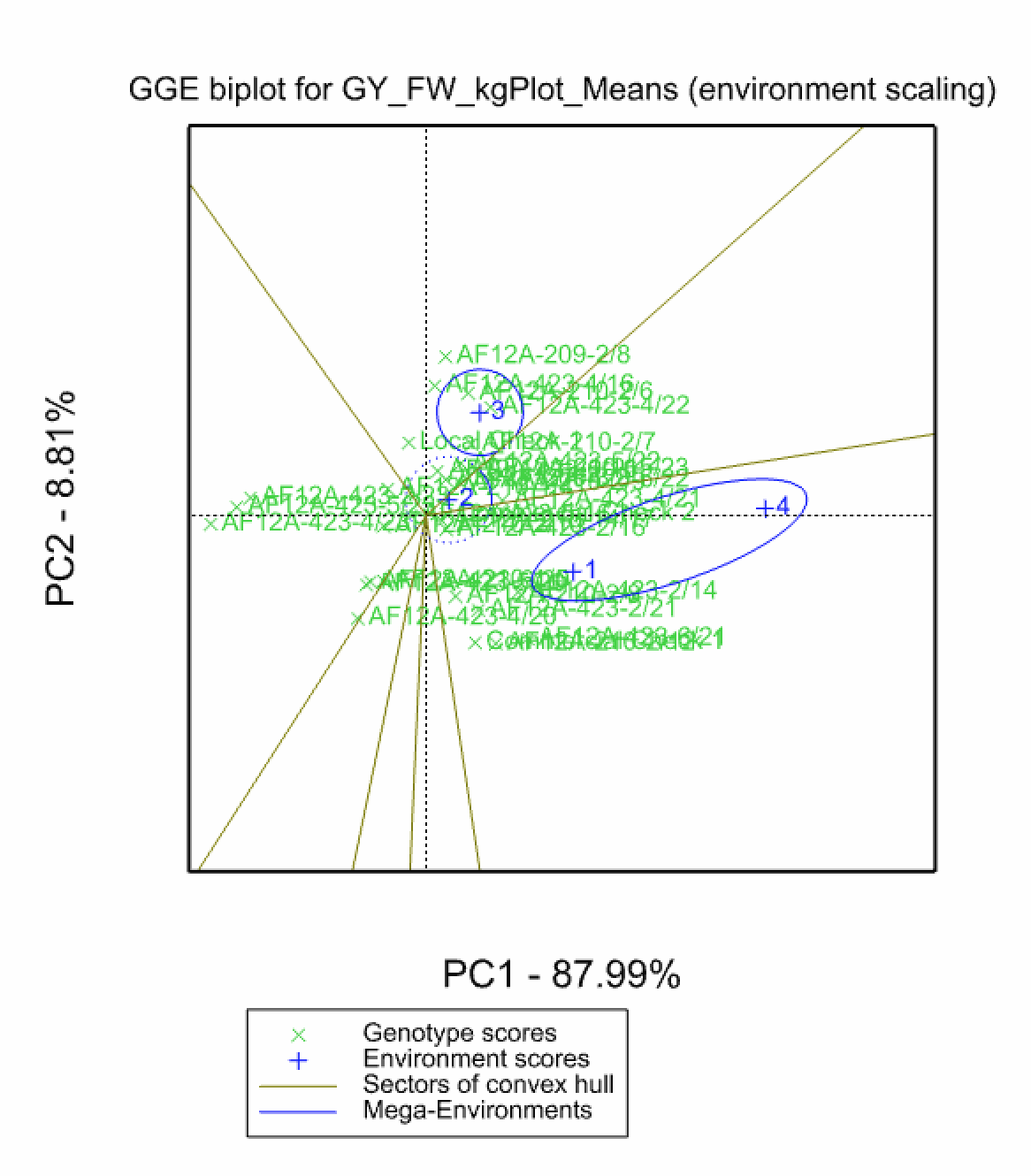
Environments 1 & 4 cluster, indicating that these two locations have similar environmental effects on phenotype and small GxE interactions.
Variance-Covariance Model & Correlation Matrix
Details on the variance-covariance model, including the pairwise correlation matrix from the covariance model is presented in a table in the Report tab. In the correlation matrix values close to 1 indicate higher correlation between environments. A value of 1 indicates a perfect correlation, such as when an environment is compared to itself.
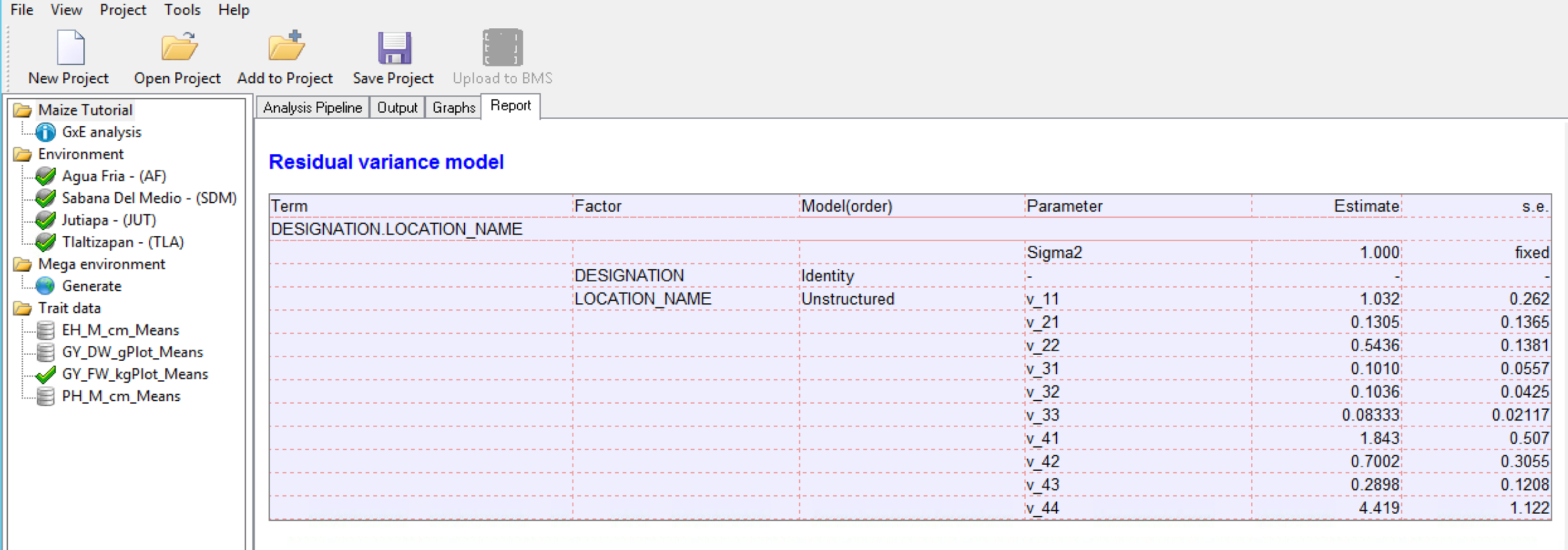
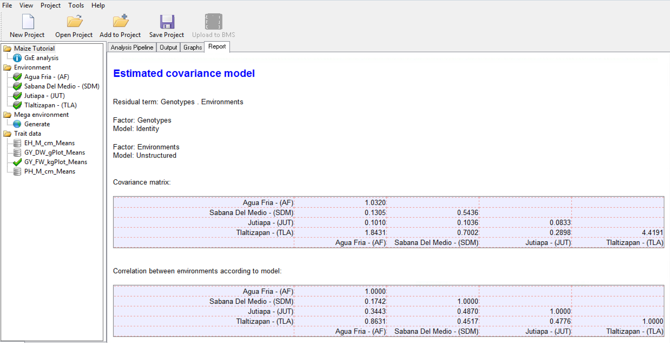
Correlation Matrix for Grain Yield (GY_FW_kgPlot): Environment 1 is most positively correlated to the Environment 4 (0.8631), suggesting that the two locations have similar environmental effects on phenotype.
Correlation Heat Map
The correlation heat matrix visualizes correlations with color; warm colors (red) indicating high positive correlation between environments, and cool colors (blue) indicating high negative correlation between environments.
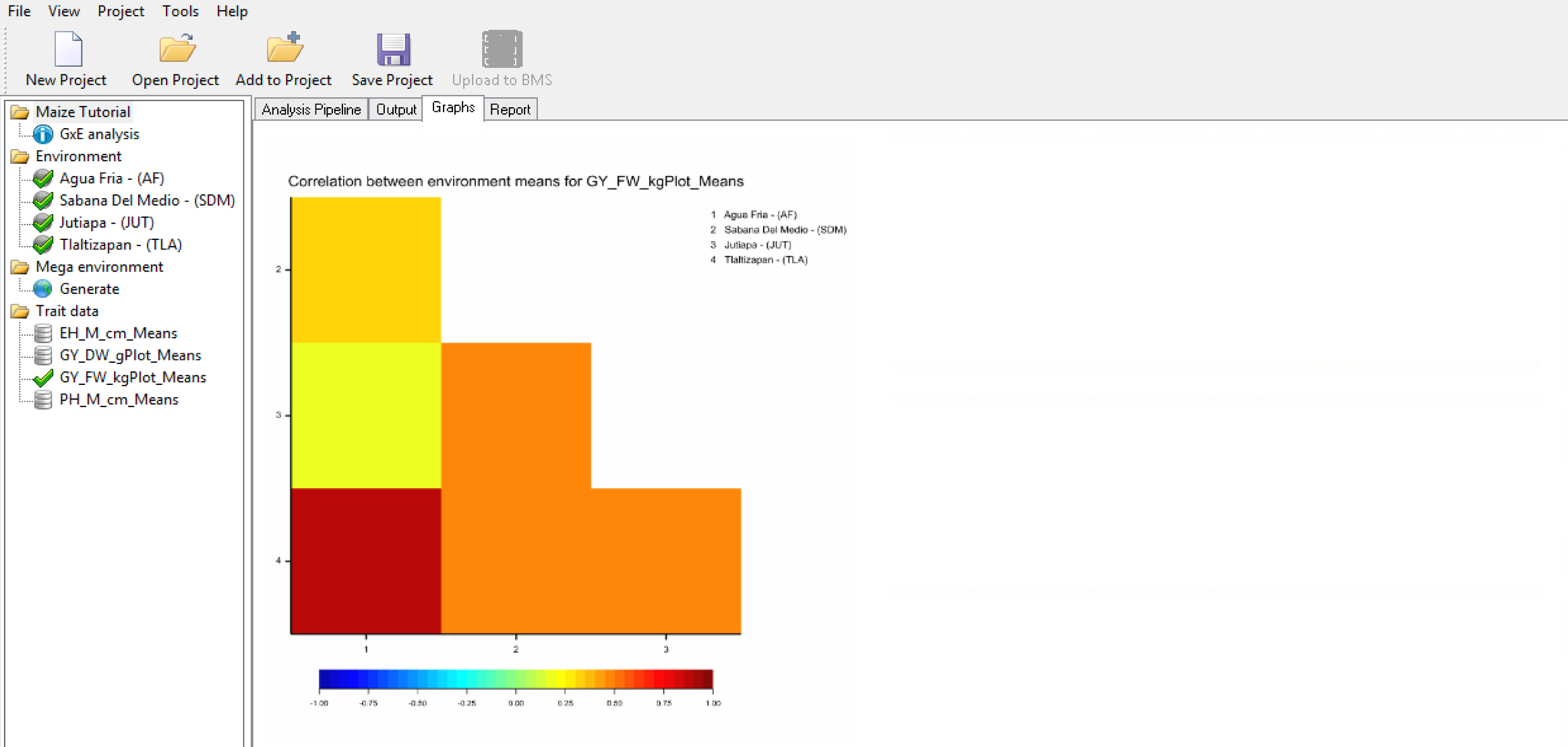
Correlation Heat Map of Grain Yield (GY_FW_kgPlot): Environment 1 is most positively correlated (red) to Environment 4 environment, suggesting that these two locations have similar environmental effects on phenotype and small GxE interactions.
Scatter Plot Matrix
The scatter plot matrix illustrates the association of genotypic performance between each pair of environments.
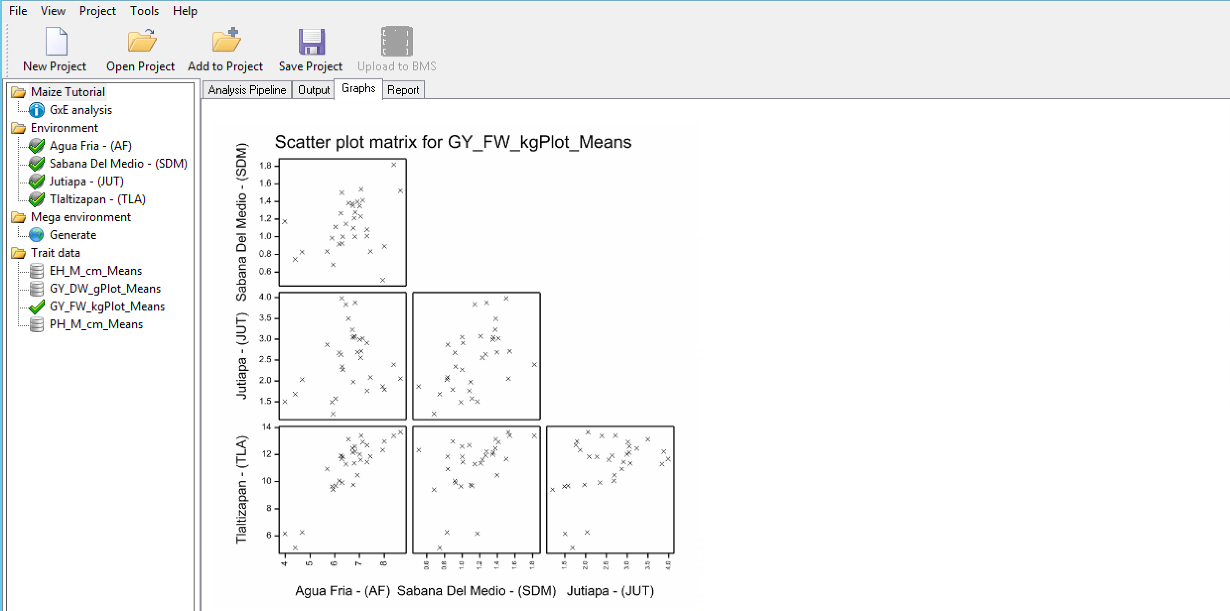
Scatter Plot Matrix for Grain Yield (GY_FW_kgPlot): A positive correlation is observed between genotypic performance at Environments 1 & 4 indicating similar environmental effects on phenotype for these environments and small GxE interactions. However, little correlation is observed between genotypic performance at Environment 1 and 3, indicating large GxE interactions between these two environments.
References
Gauch, H. G. (1988). Model selection and validation for yield trials with interaction. Biometrics, 44, 705–715.
Gauch, H.G. (1992). Statistical Analysis of Regional Yield Trials – AMMI analysis of factorial designs. Elsevier, Amsterdam.
Finlay, K.W. & Wilkinson, G.N. (1963). The analysis of adaptation in a plant-breeding programme. Australian Journal of Agricultural Research, 14, 742-754.
Murray, D. Payne, R, & Zhang, Z. (2014) Breeding View, a Visual Tool for Running Analytical Pipelines: User Guide. VSN International Ltd. (.pdf) (Sample data .zip).
Lin, C.S. & Binns. M.R. (1988). A superiority performance measure of cultivar performance for cultivar x location data. Canadian Journal of Plant Science, 68, 193-198.
Lin, C. S., Binns, M. R., & Lefkovitch, L. P. (1986). Stability analysis: Where do we stand? Crop Science, 26, 894–900.
Oakey, H., Verbyla, A. P., Pitchford, W., Cullis, B., & Kuchel, H. (2006). Joint modeling of additive and non-additive genetic line effects in single field trials. Theoretical and Applied Genetics, 113, 809–819.
Wricke, G. (1962). Uber eine method zur erfassung der okogischen streubreite in feldversuchen. Zeitschriff Fur Pflanzenzuchtung, 47, 92-96.
Yan, W., Hunt, L. A., Sheng, Q., & Szlavnics, Z. (2000). Cultivar Evaluation and Mega-Environment Investigation Based on the GGE Biplot. Crop Science, 40, 597–605.
Yan, W. & Kang, M.S. (2003). GGE Biplot Analysis: a Graphical Tool for Breeders, Geneticists and Agronomists. CRC Press, Boca Raton.
Yan, W., Kang, M.S. Ma, B., Woods, S., Cornelius, P.L. (2007) GGE Biplot vs. AMMI Analysis of Genotype-by-Environment Data. Crop Science. 47, 643–653.
Related Materials
Manual: Manage Trials
Maize Tutorial: Trial Design & Data Collection
Maize Tutorial: Single Site Analysis: 4 Location Batch
The Integrated Breeding Platform (IBP) is jointly funded by: the Bill and Melinda Gates Foundation, the European Commission, United Kingdom's Department for International Development, CGIAR, the Swiss Agency for Development and Cooperation, and the CGIAR Fund Council. Coordinated by the Generation Challenge Program the Integrated Breeding Platform represents a diverse group of partners; including CGIAR Centers, national agricultural research institutes, and universities.
The statistical algorithms in the Breeding View were developed by VSNInternational Ltd in collaboration with the Biometris group at University of Wageningen. Maize demonstration data was provided by Mike Olsen from CIMMYT, the International Center for Maize and Wheat Improvement, breeding program. These data have been adapted for training purposes. Any misrepresentation of the raw breeding data is the solely the responsibility of the IBP.

This work is licensed under a Creative Commons Attribution-ShareAlike 4.0 International License


