• Data Collection
  • Data Entry: User Interface
  • Data Entry: Study Book File
    • Export File
    • Edit File
    • Import File
    • Pending
    • Accepted
• Execute Calculated Variables
• Graphical Filtering

Data Collection

The BMS permits data upload 3 different ways: (1) inline editing through the user interface, (2) Study Book file (.xls or .csv) export/import, and (3) directly from BrAPI enabled applications. This tutorial will cover data entry though the user interface and via Study Book file.

Data Entry: User Interface

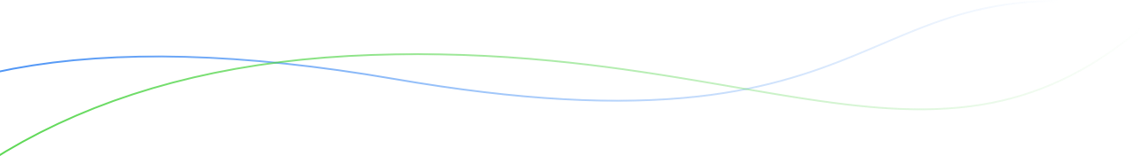
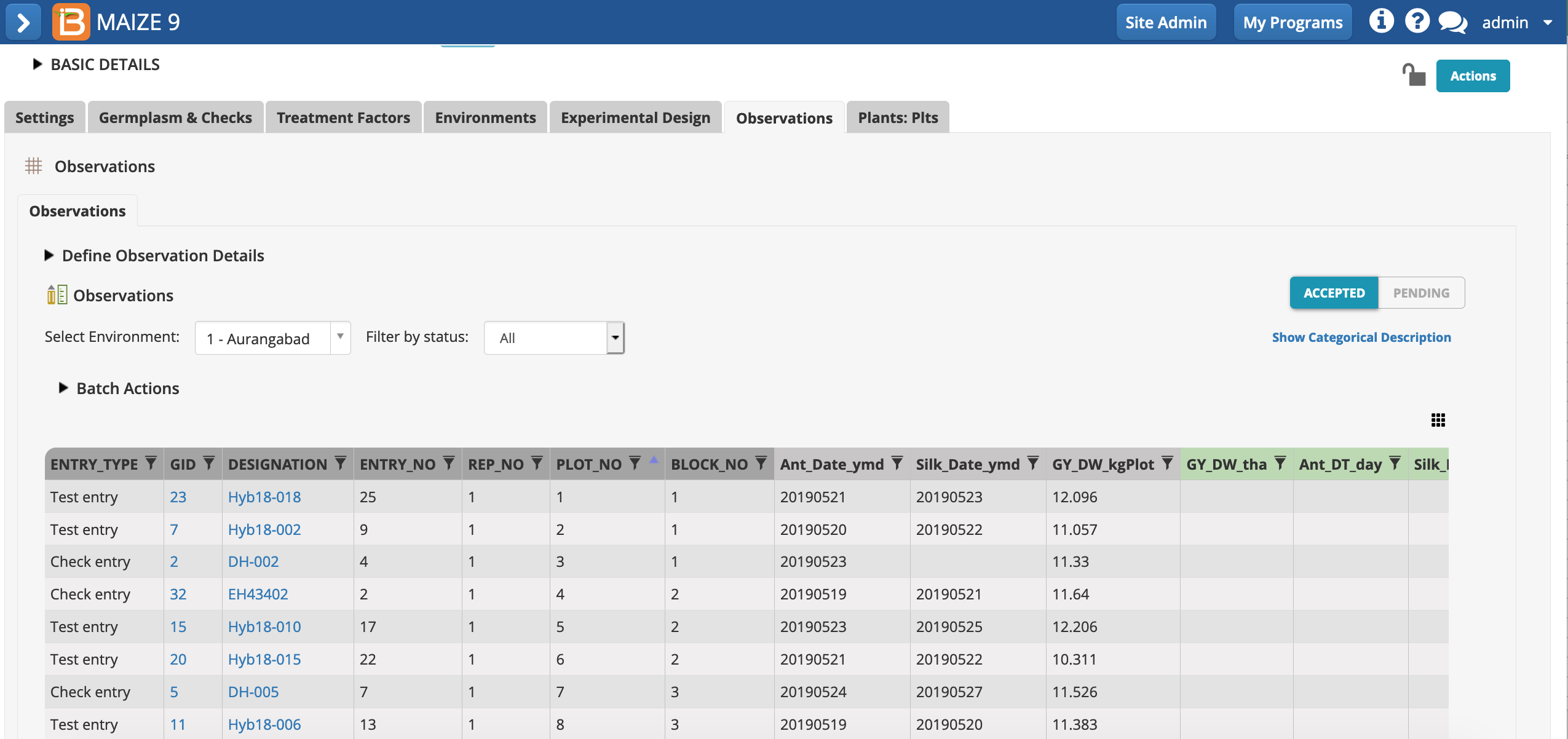
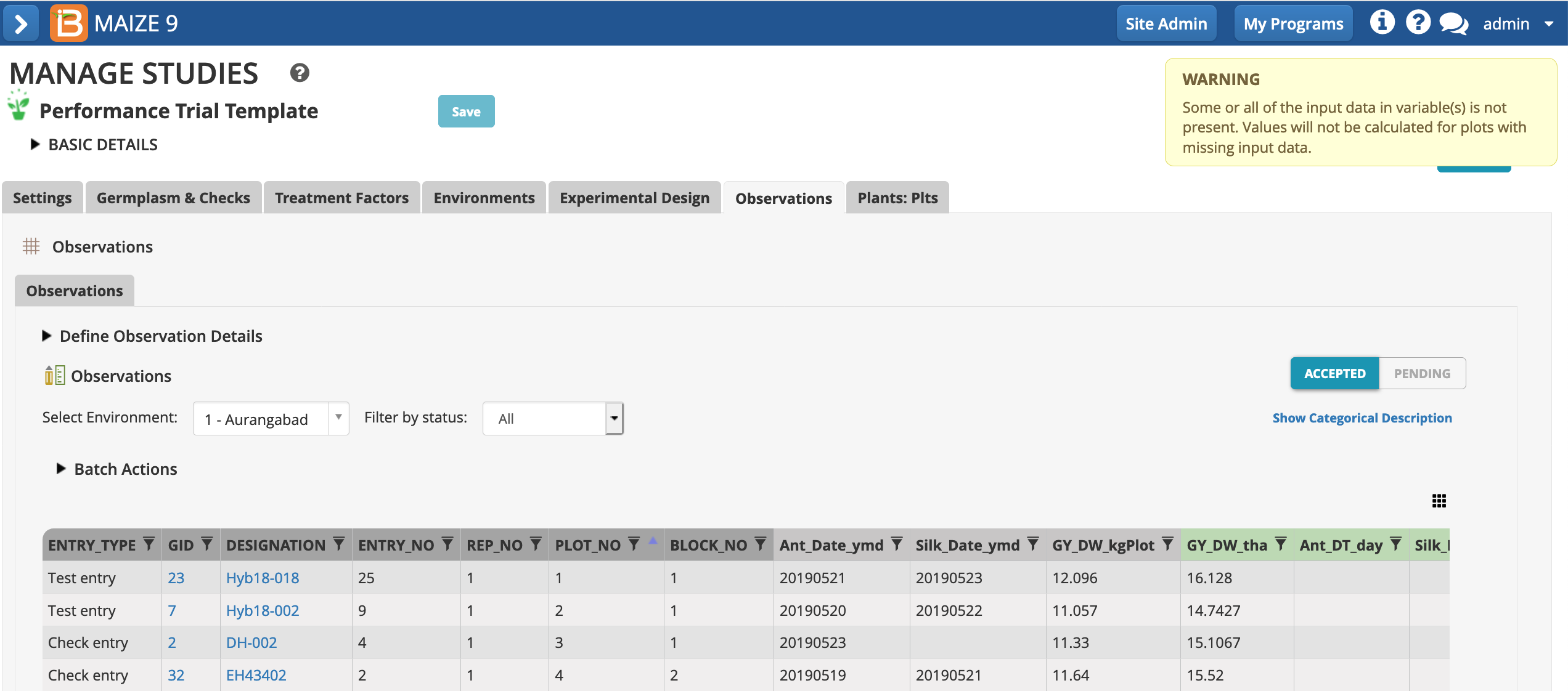
Measurements can be directly entered into the observations and sub-observations table by user interface inline editing.

• For the first plot of environment 1, enter fictional dates for anthesis and silking (yyyyymmdd) and a dry weight (kg/plot) measurement. Notice that inline edits are automatically accepted once the cursor is no longer active in the cell - this behavior differs from file and BrAPI uploads, where data is first reviewed in Pending mode.

Notice that the germplasm in plot 1, Hyb18-018 may not match the designation in your observations table, because every experimental design is an independent randomization.

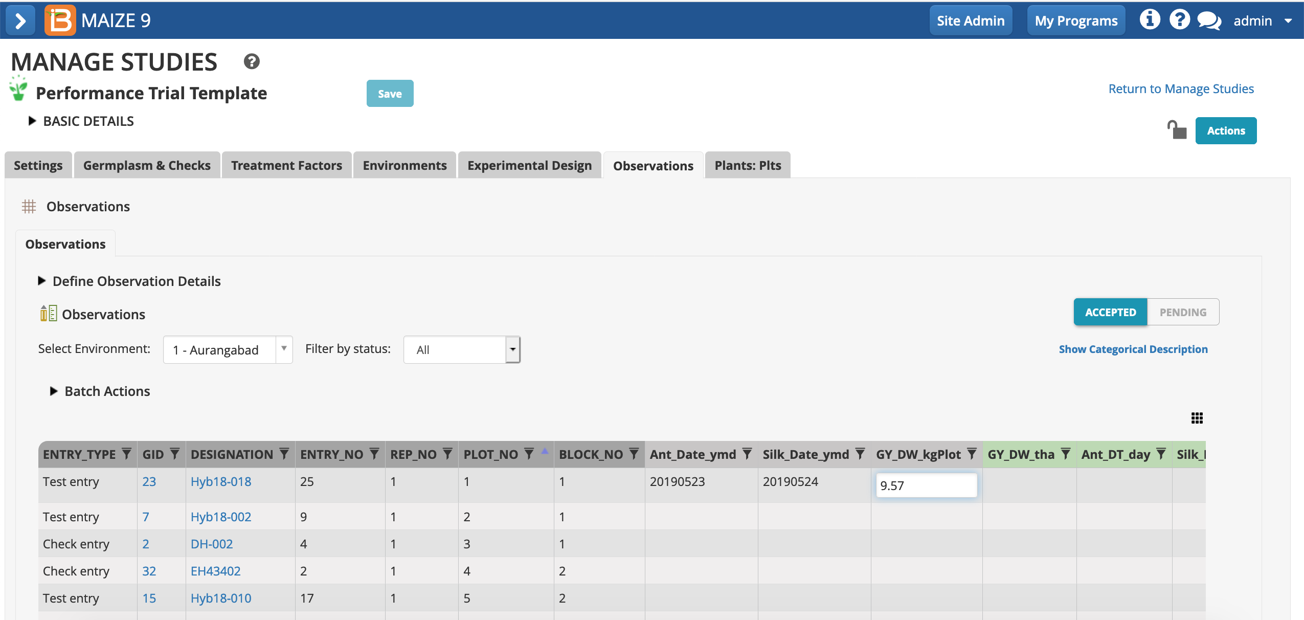
• Enter fictional data for plant and ear height in plant-level sub-observations table. Add 5 values for plant height and 4 values for ear height. These raw data values are now available for plot-level means calculations.

Data Entry: Study Book File

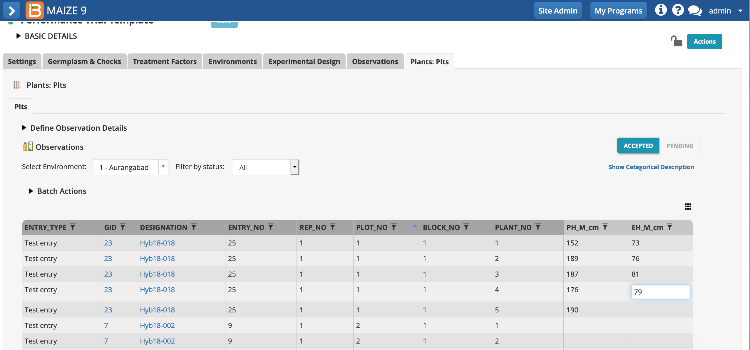
The BMS will export study observation and sub-observation datasets as files (.xls and.csv), allowing data entry using external applications, like spreadsheet or mobile data collection apps. Data uploaded via files, or BrAPI enabled apps, pends breeder review before it is accepted to the database and available for queries and analysis.

Export File

• Choose Export study book from the Actions menu.

• Continue with the Observations plot-level dataset.

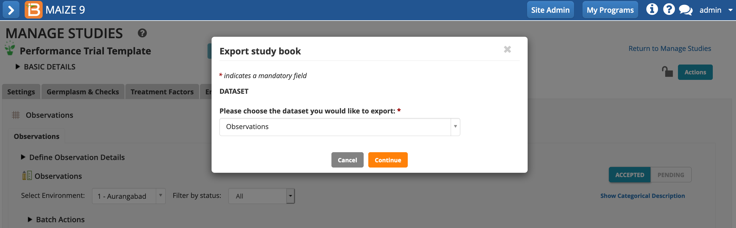
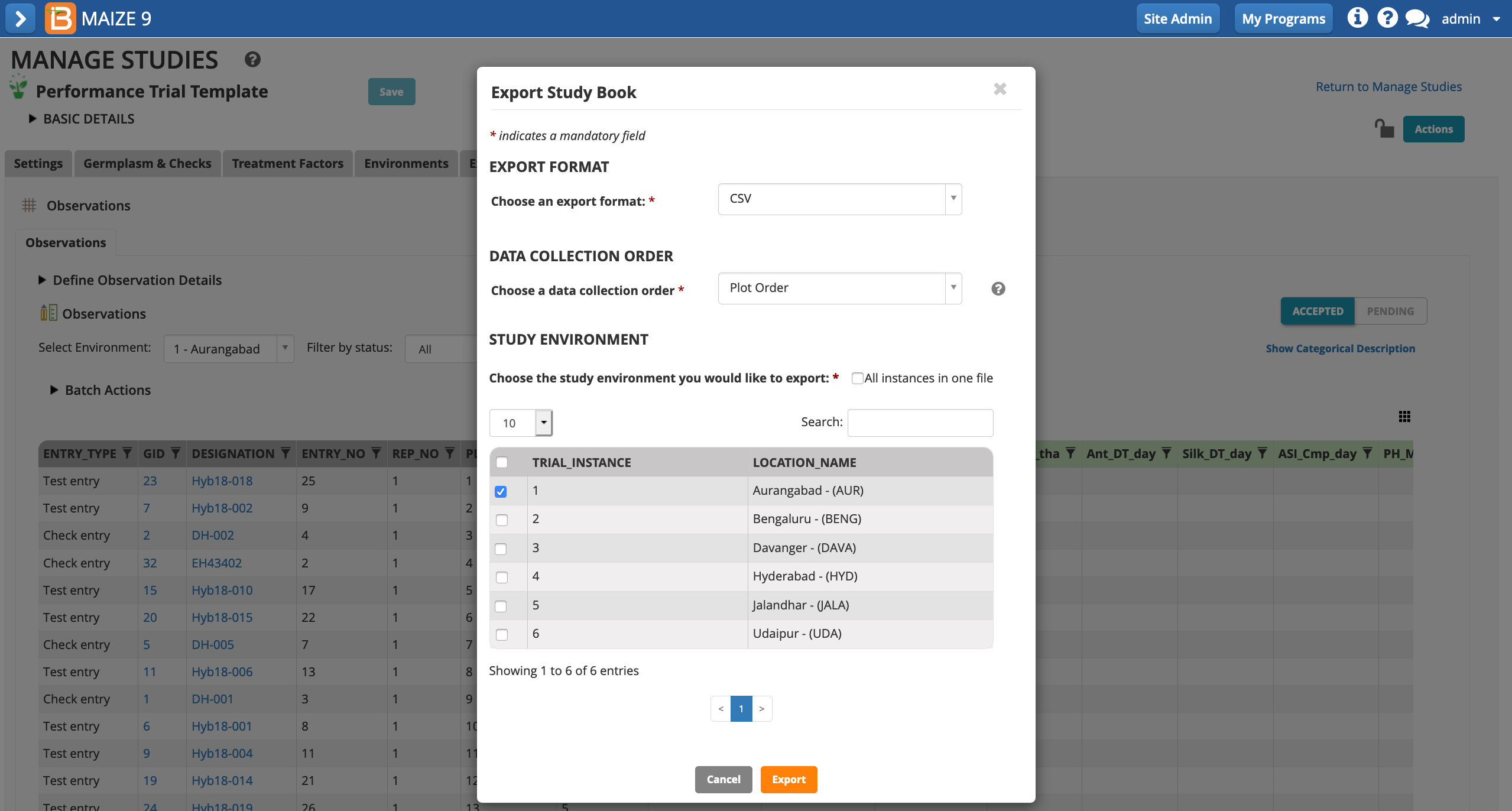
• Export only the Aurangabad location (instance 1) in .csv format.

Edit File

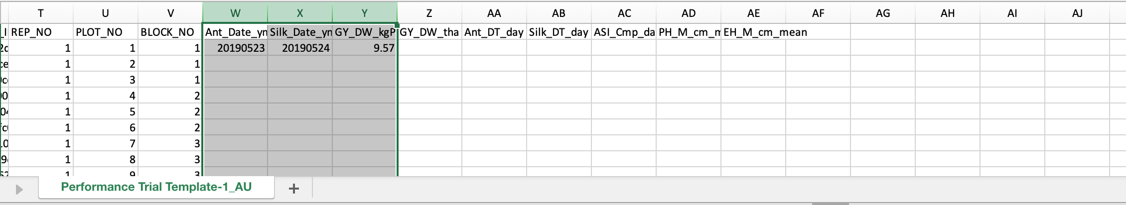
• Open the .csv file with a spreadsheet program, like Excel. Notice that the spreadsheet reflects the observations table. The columns of trait data can be edited and used to overwrite existing data. Fill the "raw" data variables with fictional data. You can make up your own data or copy and paste example data.
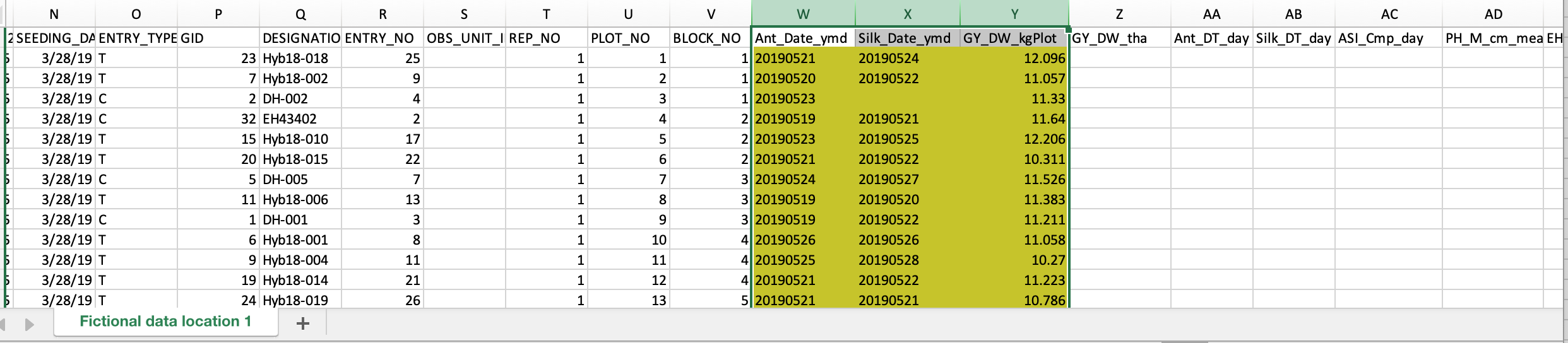
• Copy the example data highlighted in yellow and paste into your BMS export file. The BMS matches observation data by OBS_UNIT_ID. These IDs are unique to every study. You must have the correct OBS_UNIT_ID or the data will not import successfully. Save the edited file.

Example data provided in this file (.csv) is entirely fictional and meant only to serve as demonstration of data import via .csv file.

Import File

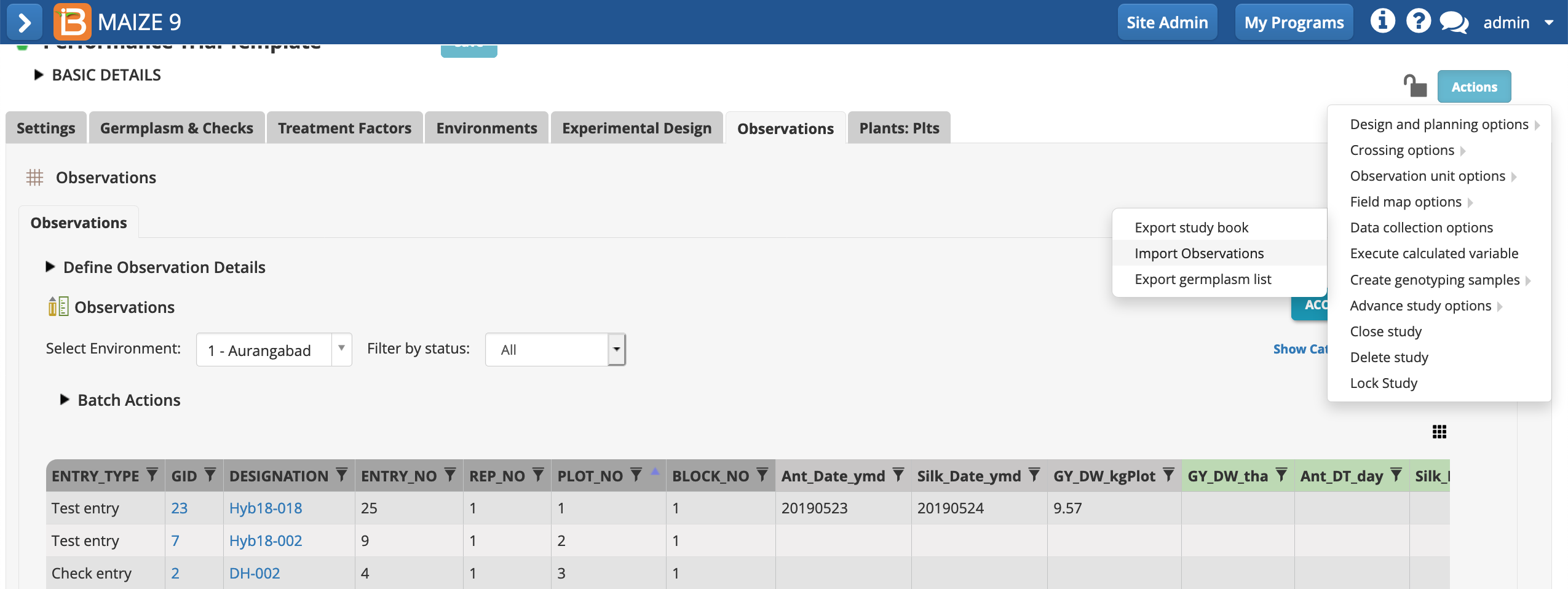
• Choose Import Observations > Data collection options > Actions menu.

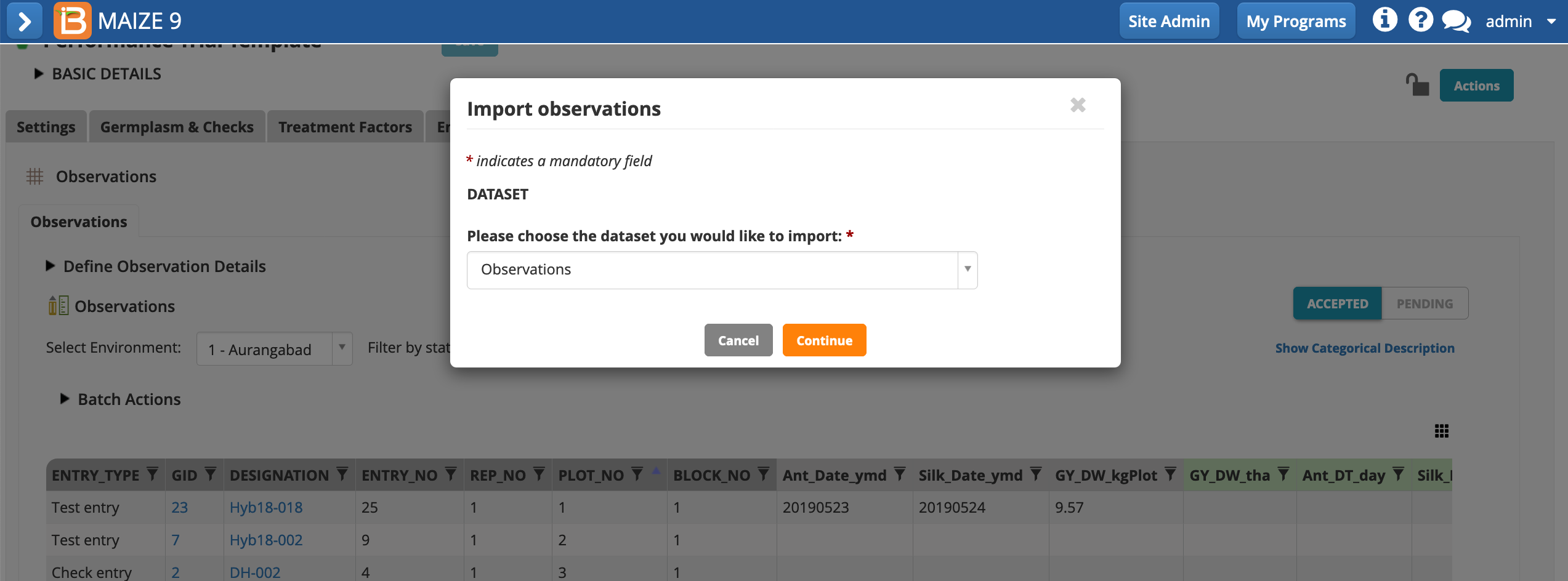
• Continue with Observations dataset.

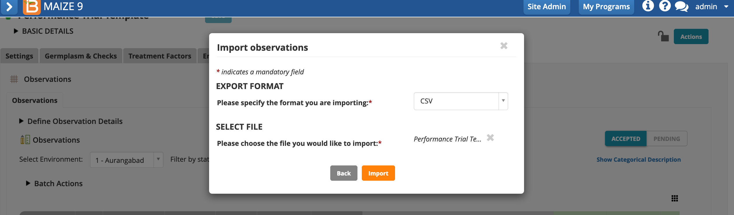
• Specify .csv file format and select the file with fictional data and your OBS_UNIT_IDs. Import.

Pending

Pending data requires breeder review, and is a quality control step to avoid accidental or malicious data errors. Only after data is accepted, is it available for queries, and calculations.

• Review the pending data. Filter by environment or status. Accept.

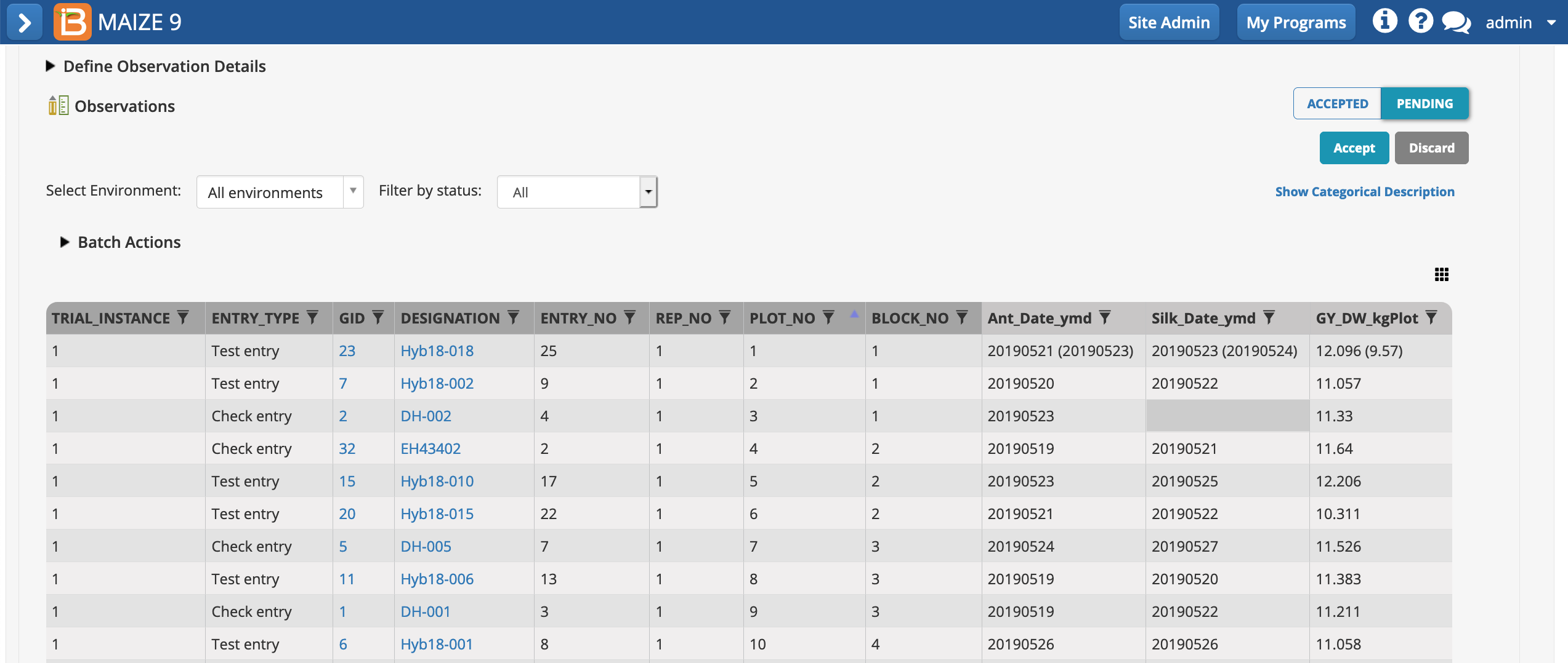
Pending data: Data for all 3 traits in plot 1 is pending overwrite (the previously accepted data are in parentheses). Silking date was not recorded in plot 3. The blank cell is highlighted grey to denote missing data.

Accepted

Accepted data is available for queries, analysis, and calculations.

Execute Calculated Variables

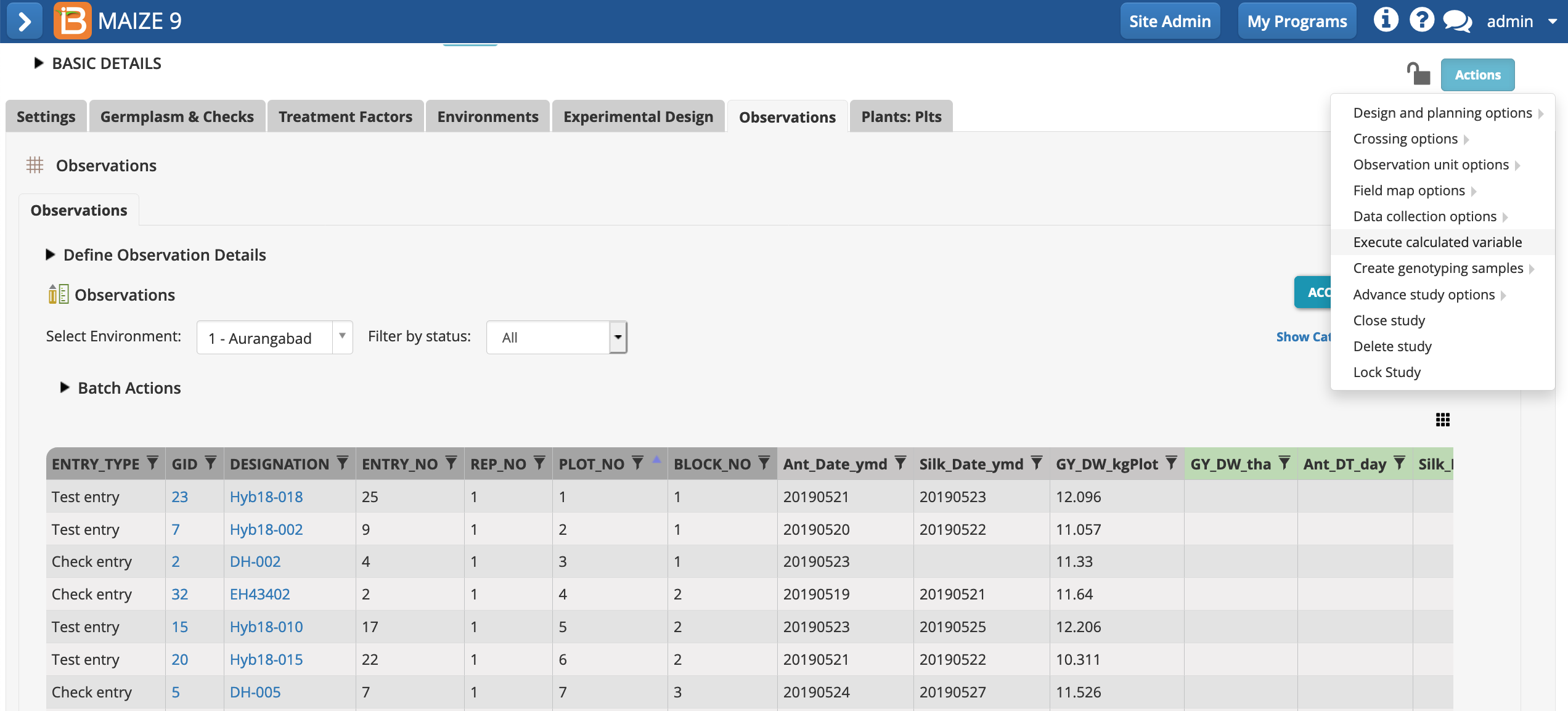
• Once the "raw" plot-level data is entered, plot-level calculations can be made. Select Execute calculated variable from the Actions menu.

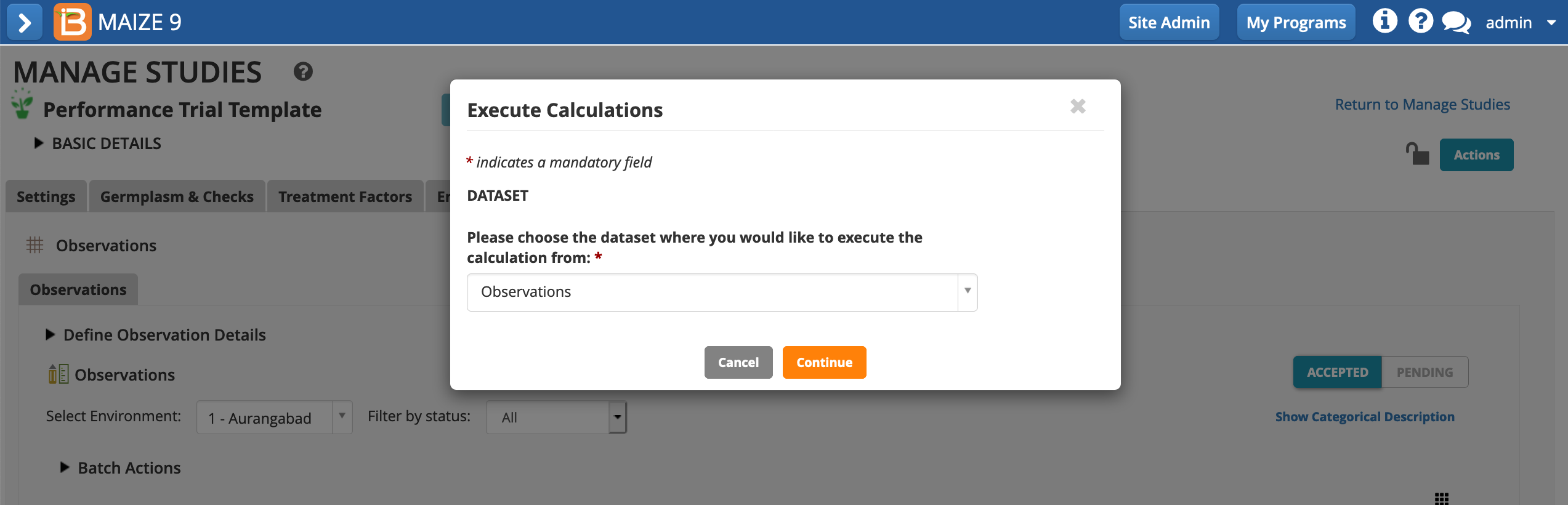
• Continue calculating from the Observations plot-level dataset.

• Choose to calculate the GY_DW_tha. The default setting, calculating all locations/instances, can be left in place. All cells with missing input data will be ignored. Execute calculation.

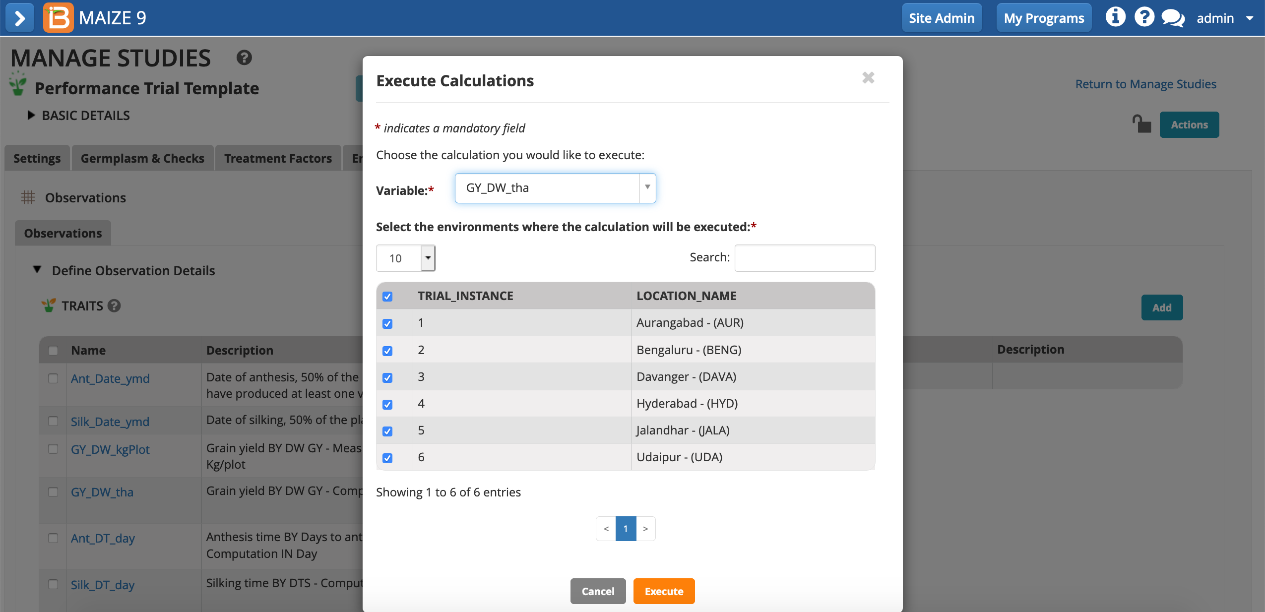
The dry weight grain yield (t/h) has been calculated by the BMS using plot size (m²) and dry weight grain yield (kg/plot). Because we are entering only data for one location of the study, a warning message alerts that not all cells could be calculated due to missing data.

• Repeat the calculations for the other 5 derived variables.

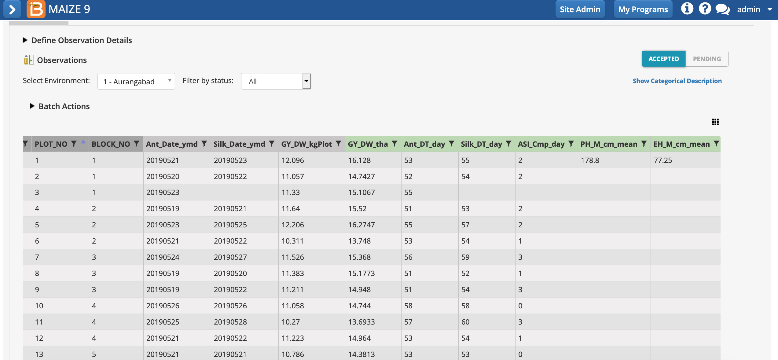
Notice the missing data. Silking date was not recorded for plot 3, so days to silking and anthesis/silking interval could not be calculated and are blank cells. Plant and ear height means are only calculated for plot 1, because no sub-observations are recorded at other plots.

Graphical Filtering

At this point the study is ready to receive the rest of the plot-level observations for other locations and the rest of the plant-level height measurements. However, a few traits measured at location 1, Aurangabad are ready for closer examination.

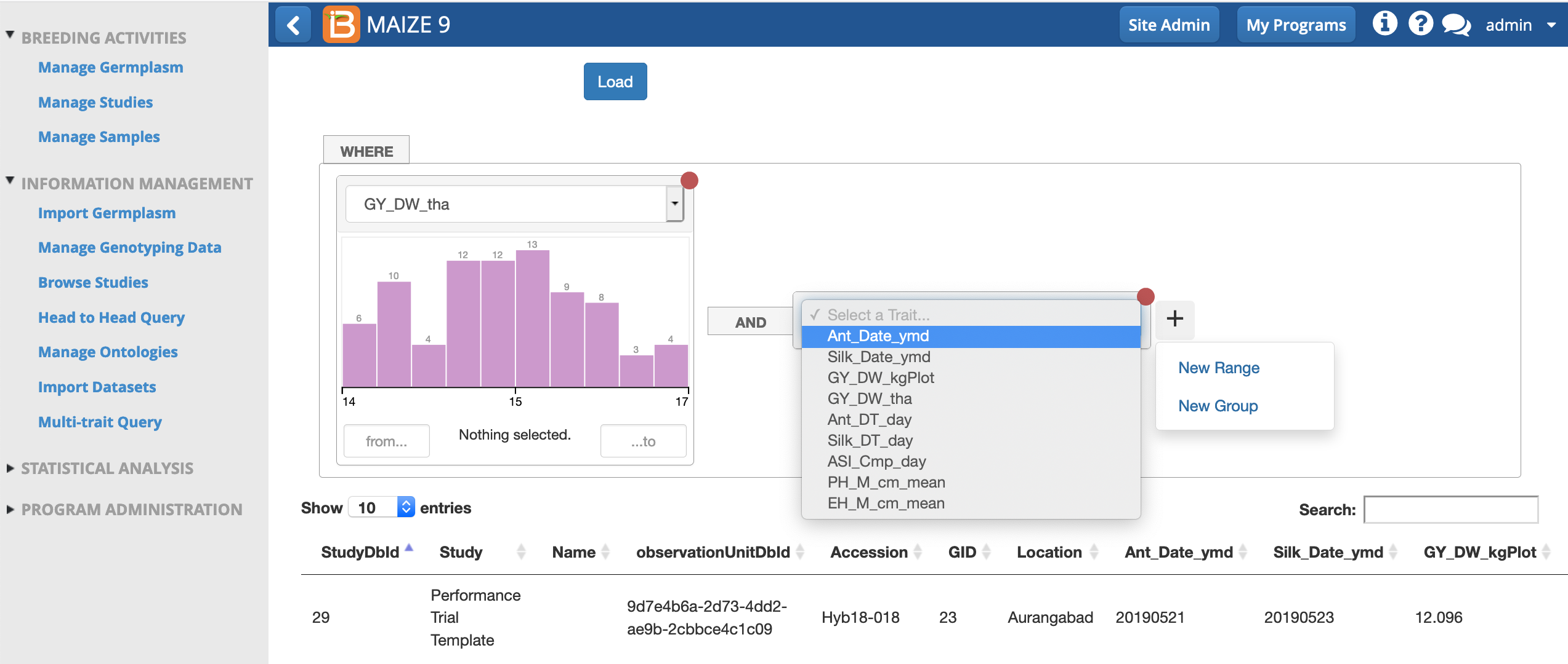
• Under Information Management, go to Browse Studies and select the Graphical Filtering Tool.

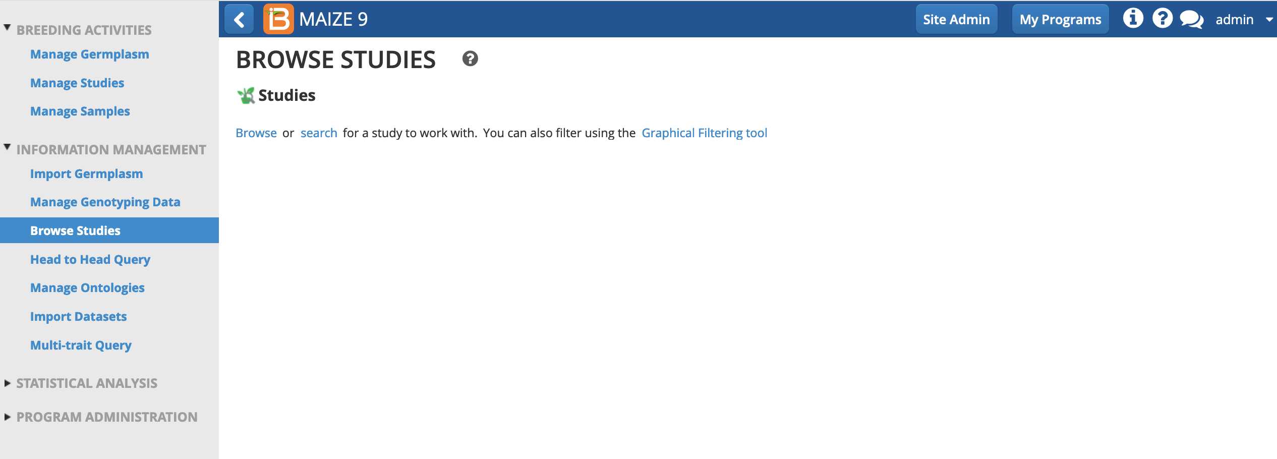
• Select the Study Name and Observation level, plot. Load.

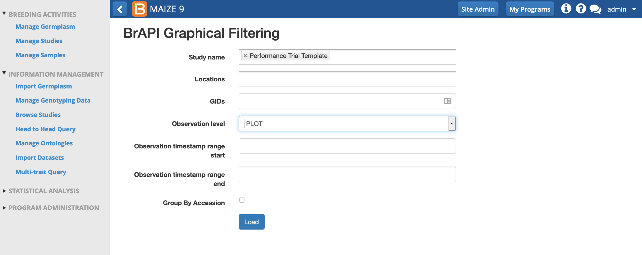
• Add two new ranges corresponding to the traits GY_DW_tha and Ant_DT_day to reveal data histograms.

• Use the cursor to select the highest yielding and earliest flowering hybrids in this study.

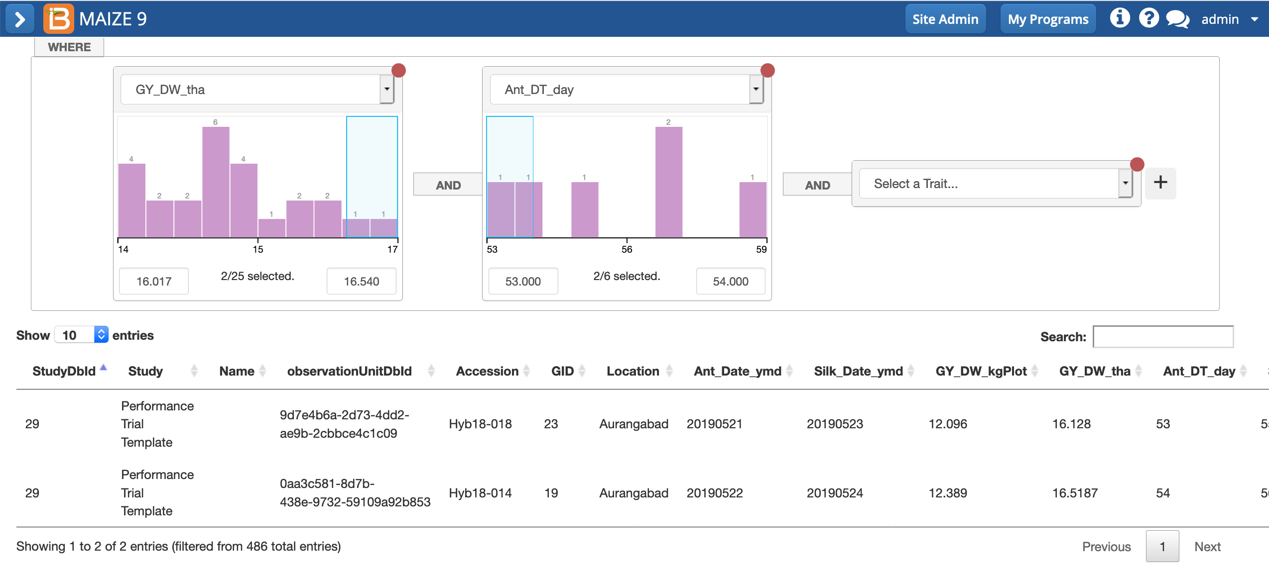
Two hybrids, Hyb19-018 and Hyb18014, are represented with high yields and early flowering. Remember that due to differences in randomization, these same hybrids might be assigned different example data and not match your selections.